Transcription
CT Image ReconstructionTerry PetersRobarts Research InstituteLondon Canada1
Standard X-ray ViewsStandard Radiograph acquires projections of the body, but since structures areoverlaid on each other, there is no truly three-dimensional informationavailable to the radiologist2
Cross-sectional imaging Standard X-rays form projection images Multiple planes superimposed Select “slice” by moving x-ray sourcerelative to film Simulates “focusing” of x-raysHowever, while X-rays cannot be focussed in the same manner as light (as inan optical transmission microscope for example), focussing can be simulatedthrough the relative motion of the x-ray and the recording medium3
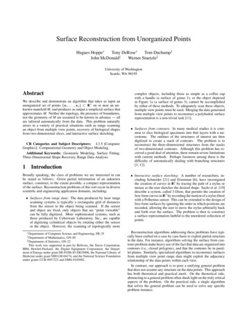
Classical TomographyXray TubeMotion of X-ray TubeStart positionEnd positionFulcrum planeAABBObject being imagedFilm End positionMotion of FilmFilm Start positionClassical longitudinal tomography used this principle. By moving the x-raytube and the film such that the central ray from the tube passes through a singlepoint in the image-plane (fulcrum plane), information from the fulcrum plane(A—A) would be imaged sharply o the film, but data from other planes (B—B)would be blurred. Thus although the desired plane was imaged sharply, it wasoverlaid with extraneous information that often obscured the important detail inthe fulcrum plane4
Transverse TomographyIf transverse sections were desired, a different geometry was required. Here thepatient and film were rotated while the x-ray tube remained fixed. However thebasic principle remained the same: the fulcrum plane was defined by theintersection of the line joining the focus of the x-ray tube, and the the centre ofrotation of the film on the pedestal.5
Transverse Tomographyx-ray sourceObject being imagedFilm planeImaged(fulcrum)planeDirection of rotationThis figure illustrates the geometry of the previous slide. Again, while thefulcrum plane is imaged sharply (because its image rotates at exactly the samerate as the film), structures from planes above and below the fulcrum plane castshadows that move with respect to the film and therefore the ima ge becomesindistinct as before.6
Transverse Tomogram ofThoraxThis techniques was known as a Layergraphy, and the image was known as alayergram. This slide shows a layergram through the thorax, and while a fewhigh contrast structures (ribs), and the lungs are visible, the image is of limiteddiagnostic use.7
x-ray sourceAperture to formlaminar beamObject being imaged(Single spot)Film planeImaged plane“Image” ofobjectDirection of rotationWhat if we change the geometry of the layergraph so that only a single planewas illuminated? For a single angle of view, a spot in the desired cross-sectionwould project a line over the film. If the object and the film were rotated asbefore, the lines would intersect on the film to give a blurred representation ofthe object.8
Projections of point objectfrom three directionsBack-projection ontoreconstruction planeFor example, after only three projections, the lines would intersect to yield a“star-pattern” 9
ObjectImagef(r)Profile through objectf(r) *1/rProfile through imageAnd after a full rotation of the film and the object, this pattern would become adiffuse blur. The nature of the blur can readily be shown to be 1/r. Thus anystructure in the cross-section is recorded on the film as a result of a convolutionof the original cross-section with the two-dimensional function 1/r.10
Let’s get Fourier Transformsout of the way first!f ( x) i 2πuxF(u)edu “forward” Fourier TransformF (u ) f ( x)e i 2πux dx “inverse” Fourier TransformSince the Fourier Transform plays a major role in the understanding of CTreconstruction, we introduce it here to define the appropriate terms.11
Reconstruction Image is object blurred by 1/r 2D FT of 1/r is 1/ρ Why not de-blur image?– 2D FT of Image– Multiply FT by ρ – Invert FT Voila!Back to the blurred layergram! If the image is blurred with a function whoseFT is well behaved, we should be able to construct a de-blurring function. Itturns out that the 2-D FT of 1/r is 1/ρ. Since the inverse of 1/ρ is ρ , then weshould be able to compute the 2D FT of the blurred image, multiply the FT ofthe result image by ρ , and then calculate the inverse FT.12
There’s morethan onescanway to skin a CATThe previous approach is certainly one approach, but not necessarily the mostefficient. There are in fact a number of different ways to view thereconstruction process.13
Central Slice Theorem Pivotal to understanding of CTreconstruction Relates 2D FT of image to 1D FT of itsprojection N.B. 2D FT is “k-space” of MRIOne of the most fundamental concepts in CT image reconstruction if the“Central-slice” theorem. This theorem states that the 1-D FT of the projectionof an object is the same as the values of the 2-D FT of the object along a linedrawn through the center of the 2-D FT plane. Note that the 2-D Fourier planeis the same as K-space in MR reconstruction.14
Central Slice Theorem2D FTφProjection at angleφ1D FT of Projection at angle φThe 1-D projection of the object, measured at angle φ, is the same as theprofile through the 2D FT of the object, at the same angle. Note that theprojection is actually proportional to exp (- u(x)xdx) rather than the trueprojection u(x)xdx, but the latter value can be obtained by taking the log ofthe measured value.15
Horizontal Projection2-D Inverse FT1-D Fourier TransformVertical ProjectionInterpolate in FourierTransform1-D Fourier Transform2-D Fourier TransformIf all of the projections of the object are transformed like this, and interpolatedinto a 2-D Fourier plane, we can reconstruct the full 2-D FT of the object. Theobject is then reconstructed using a 2-D inverse Fourier Transform.16
Filtered Back-projection Direct back-projection results in blurredimage Could filter (de-convolve) resulting 2-Dimage Linear systems theory suggests order ofoperations unimportant Filter projection profiles prior to backprojectionYet another alternative, (and the one that is almost universally employed)employs the concept of de-blurring, but filters the projections prior to backprojection. Since the system is linear, the order in which these operations areemployed is immaterial.17
Convolution FilterIn Fourier Space, filter has the form ρ Maximum frequency must be truncated at ρ’Filtering may occur in Fourier or Spatial domain ρ’0ρ’Frequency response of filterρSampled convolution filterSince the Fourier form of the filter was already shown to be ρ , the spatialform is the inverse FT of this function. The precise nature depends on thenature of the roll-off that is applied in Fourier space, but the net result is aspatial domain function that has a positive delta-function flanked by negative“tails”18
Result is Modified(filtered) projectionIFTFT X ρ Original projectionof pointMultiply FourierTransform by ρ Compute FourierTransform of projection Compute inverseFourier TransformOR convolve withIFT of aboveHence we can take the projection of the cross-section, shown here as a singlepoint, and either perform the processing in the Fourier domain throughmultiplication with ρ , or on the spatial domain by convolving the projectionwith the IFT of ρ . This turns the projection into a “filtered” projection, withnegative side-lobes. It is in fact a spatial-frequency-enhanced version of theoriginal projection, with the high-frequency boost being exactly equal to thehigh-frequency attenuation that is applied during the process of backprojection.19
Back-projecting the FilteredProjectionIf we now perform the same operation that we performed earlier with theunfiltered projection, we see that the positive parts of the ima ge re-enforceeach other, as do the negative components, but that the positive and negativecomponents tend to cancel each other out.20
Back-projecting the FilteredProjectionAfter a large number of back-projection operations, we are left with everythingcancelling, except for the intensities at the position of the original spot. Whilethis procedure is demonstrated here with a single point in the cross-section,since a arbitrary projection is the sum of a large number of such points, andsince the system is linear, we can state that the same operation of a largenumber of arbitrary projections will result in a reconstruction of the entirecross-section.21
Back-project filteredprojections (at all angles)Cross-section of headFTVertical projectionof this cross-section ρ Inv FTModified (filtered) projectionReconstruction Demo22
The Mathematics of CT ImageReconstructionReconstructed imageπ g ( r, θ ) Original projections [ f (ξ ,φ )e i 2πρξ dξ ] ρ ei 2πρ r cos(θ φ )d ρ dφ0 FT of projections at each angle Multiply by ρ Invert Fourier TransformBack-project for each angleThe mathematics of the image reconstruction process, can be expressedcompactly in the above equation, where the terms have been grouped to reflectthe “filtered-back-projection” approach23
What happens to the DCterm? After “ρ” filtering, DC component of FTis set to zero Average value of reconstructed image iszero!!! But CT images are reconstructed withnon-zero averages! Huh?A conceptual problem arises with this approach though. If we are filtering theFourier Transform of the mage by multiplying it by the modulus of the spatialfrequency, then we explicitly multiply the zero frequency term (the “DC”term) by zero. This implies that the reconstructed image has an average valueof zero! And yet the reconstructed images always in fact have their correctvalue. What’s up?24
Side-step to convolutiontheorya f(x)a bb g(x)f(x) g(x)To explain the apparent paradox, we need to revisit an important aspect ofconvolution theory. When two function are convolved, the result of thisoperation has a support equal to the sum of the supports of the individualfunctions. It doesn’t matter whether the operation has been carried out in theimage domain or the Fourier domain: the result is the same.25
DC Term?Extent of original projection Reconstructed image indeed has average .value of zero Only central part of interest Reconstruction procedure ignores values .outside FOV All is well!Extent of projection after filtering- ---So turning back to our reconstruction example, the full reconstructed image(which actually has a support diameter of double that of the originalprojections), indeed has an average value of zero (this is what setting the“DC” term in Fourier domain to zero implies), but that the part of the imagethat is of interest (i.e. the original field-of-view defined by the projections)contains exactly the correct positive values. It is the surrounding annulus (thatis of no interest) that contains the negative values that exactly cancel thepositive values in the center. Note that the outer annulus does not have to beexplicitely computed, and so it is seldom apparent.26
Projections to ImagesProjections1D FTBack-Project1D FT2D FTx 2D Rho-filterInterpolate into 2DFourier Space 1D Rho-filter2D IFT1D IFT2D IFTBack-ProjectImageSo there are multiple routes to arrive at an image from its projections.27
SinogramξScanned ObjectProjection DataφφφAnother concept that is useful to use when considering CT reconstruction isthe “Sinogram”, which is simply the 2-D array of data containing theprojections. Typically, if we collect the projections, using a hypotheticalparallel-beam scanning arrangement, using φ as the angular parameter and ξas the distance along the projection direction, we refer to the (φ, ξ) planerepresentation of the data as the “sinogram”.28
Projection GeometriesParallel-beam configurationFan-beam configurationφξIt is worth pointing out that there are two common geometries for datacollection; namely parallel-beam and diverging-beam. The parallel-beamgeometry was once used in practical scanners, while the diverging-geometry isemployed exclusively today. The parallel-beam configuration is useful explainthe concepts; allows simpler reconstruction algorithms, and is often the form towhich diverging-ray data are converted prior to image-reconstruction.29
3rd and 4th GenerationSystemsBoth 3rd and 4th generation systems employ diverging-ray geometry30
¼ Detector Offset In 3rd generation fan-beam geometry, detector width detector spacing. Should sample 2x per detector width (Nyquist) Symmetrical configuration violates this requirement ¼ offset achieves appropriate sampling at no cost Symmetrical detector– 180 fan angle ¼ Det offset– 360 to fill sinogramThere is a fundamental problem with 3rd generation geometries, where thedetector width is effectively the same as the sampling width. In theory thesampling should be equal to half the detector width, bit this is clearlyimpossible with the 3rd generation geometry. However the simple technique ofoffsetting the detector array from the centre of rotation by ¼ of the detectorwidth achieves effectively the appropriate sampling strategy31
No Detector Offset180 0 Rotate about point on central rayIf we rotate a 3rd generation system about the central ray, it is clear thatdetectors symmetrically placed about the central detector, mostly “see” thesame annulus of data in the image.32
No Detector Offset Symmetrical pairs ofdetectors “see”same ring in object Minor detectorimbalance leads tosignificant “ringartefact”.Rotate about point on central rayAs we rotate the gantry through 180 deg, these pairs respond mainly to datalying on rings. Incidentally, detector imbalance generates “ring-artefacts” inthe images.33
With ¼ -detector Offset Note red and green circlesnow interleaved – sinogramsampling is doubled!0 180 Rotate about point ¼ det spacing from central rayHowever, if we offset the detector by ¼ of the detector spacing, we see that thesame pairs of detectors now see different annuli. Thus we have effectivelydoubled the sampling without any cost to the system except that we must scanthe full 360 degrees, rather that the 180 deg fan angle that is all that isnecessary with the symmetrical configuration.34
Reconstruction from Fanbeam data Interpolate diverging projection data intoparallel-beam sinogram Adapt parallel-beam back-projectionformula to account for diverging beam– weighting of data along projection tocompensate for non-uniform ray-spacing– inverse quadratic weighting in backprojection to compensate for decreasedray-spacing towards source.If we have data from a fan-beam geometry system (highly likely with today’sscanners), we can do either of two things. Firstly we can recognise that everyray in a fan-bean has an equivalent ray in a parallel-beam configuration, andsimply interpolate into a parallel-beam sinogram prior to image reconstruction.Or we can adapt the reconstruction formulae to reflect the diverging-ray, ratherthan the parallel-ray data.35
Fan-beam ReconstructionActual Detector ArcEquivalent Linear DetectorThere are two aspects to these formula modifications. First we observe that theequi-spaced data collected on an are are the same as non-linearly –space datacollected along a linear detector. We therefore multiply the projection dataelements with a 1/cosine weighting factor to reflect this fact.36
Diverging BeamReconstructionWeight back-projectionto account for converging raysWeight convolution toto account for non-linear samplingThen perform diverging-ray back-projection as beforeAlso, since the rays become closer together as they approach the source, wemust incorporate an inverse quadratic weighting factor in the back-projectionto account for this “bunching-up” of the rays.37
Projection GeometriesFan-beam configurationParallel-beam configurationξξφθψRay defined by θ and ψ in fan-beam is the same as that definedby ξ and φ in parallel-beam configurationBack to the two geometries. The red ray in both the parallel and divergingconfigurations are the same, and therefore occupy the same point in sinogramspace.38
Sinogramξ0φπ2πWhile the parallel-beam data fill up sinogram space in parallel rows, thediverging ray data fill up the same space along curved lines. Note thatsinogram repeats itself after 180 deg, except that the order of the individualdata elements are reversed (a consequence of the fact the projection at angle 0is the same as that at angle 180 deg, except that it is flipped). Note also thatbecause of this behavior, the data from the diverging–ray sinogram at 180 deg“wraps-around” into the sinogram at the top.39
Parallel vs Fan-beam Every ray-sum in fan-beam “sinogram”has equivalent point in parallel-beamsinogram Interpolate div ray projections intoparallel-beam sinogram Perform reconstruction as if data werecollected in parallel-beam geometryThis behaviour allows us to interpolate the diverging-ray data into a parallelray sinogram.40
Interpolating fan-data intoSinogram0Note that sinogram line forφ 0 and φ π are equivalentbut reversed in ξφRotating fan-beam detector byπ misses red areas in sinogramπξNeed to rotate extra ψ (fan angle)To collect sufficient data.Need to rotate through 2 π with ¼ detectoroffset2π41
Spiral (Helical) Scanning X-ray tube/detector rotates continuouslyPatient moves continuouslySingle or Multi-sliceFundamental requirements of CT violated– Successive projections not from same slice– Projections not self-consistent Virtual projections of required slicesinterpolated from acquired data - “Zinterpolation”Most modern scanners operate in a helical or spiral mode where the x-ray tubeand detector system rotate continuously during data acquisition as the patienttable moves through the scanner. Under these conditions, the projections arenot collected on a slice-by-slice basis, and so the reconstruction techniquesdescribed earlier cannot be used directly. However, virtual projections, (or avirtual sinogram) can be constructed for each required reconstructed slice bysuitable interpolation from the adjacent projections.42
Slice-by-slice vs HelicalSlice-by-slice approachHelical approach1-qn Pθn πP’n(z) Pθn(1-q) Pθn π (q)Angle of projectionZ - displacementPθnPθn 2πqnIn a standard CT scanner, the slice to be imaged would be moved into aparticular z position, and the gantry rotated through 360 degrees to acquire althe necessary projections. With spiral scanning, we musty, for each projectionangle, interpolate new projections from those available at z-positions differentfrom that of the reconstructed slice. The simplest approach to derive aninterpolated projection for angle θ for example, is to locate the projections forthis angle on each side of the desired slice and compute a synthesisedprojection by linear interpolation. A slightly more sophisticated approach is torecognise that points in the sinogram repeat every 180 deg /- the half the fanangle, and interpolate new rays from projections in opposite directions.43
Interpolating from spiralprojection data0Sinograms of slices tobe reconstructedπExtended sinogram ofspiral rotation projection dataπφ-πGantryRotationAngle2π Regular sinogramrepeats every π Use samples of spiralsinogram separated by πfor interpolation.2πφ3π3πSample # (along detector)4πZ-distanceAnother way or thinking about this is to imagine that the data from a helicalscanner creates an extended sinogram from which conventional sinograms atthe appropriate z intervals need to be calculated.44
Multi-slice Spiral Linear or higher-order interpolation schemescan be used Interpolation from views spaced by 180 or360 deg Reconstruction procedure similar to thatpreviously described Multi-slice detectors provide the advantage ofmultiple spiral sinograms acquiredsimultaneously For large multi-slice subtended angles, conebeam algorithms may be employed45
Cone-beam Geometry No exact reconstruction forcircular cone-beam geometry Approximate proceduresproposed by Feldcamp, Wang. Perform data weightings similarto div-ray back-projection Back-project into 3D volume Reconstructions acceptable ifcone-angle not too large Used in commercial 3Dangiograpy systemsSourceDetectorWhen the angle of beam divergence in the z direction becomes large, then theslices can no longer be considered to be parallel. Even in multi-slice detectorsthis can become a problem. In this case the back-projection must be performedalong converging rays in both directions. While there is no exactreconstruction formula for reconstructing objects from cone beam data whenthe x-ray source rotates in q plane about a fixed point, extension of themethods presented earlier nevertheless permit high quality images to bereconstructed.46
3D CTC-arms are not just for Angiography!Typical 3D cone-beam CT scanners are built around standard C-armangiographic systems.47
Summary CT reconstruction is fundamentally animage de-blurring problem The key principle is the Central SliceTheorem Of the many approaches for imagereconstruction, the convolution-backprojection method is preferred48
Summary ¼ detector offset increases sampling rate atno cost Spiral scanning techniques use interpolationto create new sinograms related to therequired slices While cone-beam reconstruction is onlyapproximate, high quality images cannevertheless be obtained by adapting fanbeam techniques to cone-beam geometry49
Pivotal to understanding of CT reconstruction Relates 2D FT of image to 1D FT of its projection N.B. 2D FT is “k-space” of MRI One of the most fundamental concepts in CT image reconstruction if the “Central-slice” theor