Transcription
Statistical Reconstruction in CTJeffrey A. FesslerEECS DepartmentUniversity of MichiganSPIE Medical Imaging WorkshopFeb. 13, 2011http://www.eecs.umich.edu/ fessler1
Full disclosure Research support from GE HealthcareResearch support to GE Global ResearchWork supported in part by NIH grant R01-HL-098686Research support from Intel2
CreditsCurrent students / post-docs Jang Hwan Cho Wonseok Huh Donghwan Kim Yong Long Madison McGaffin Sathish Ramani Stephen Schmitt Meng WuGE collaborators Jiang Hsieh Jean-Baptiste Thibault Bruno De ManCT collaborators Mitch Goodsitt, UM Ella Kazerooni, UM Neal Clinthorne, UM Paul Kinahan, UWFormer PhD students (who did/do CT) Se Young Chun, Harvard / Brigham Hugo Shi, Enthought Joonki Noh, Emory Somesh Srivastava, JHU Rongping Zeng, FDA Yingying, Zhang-O’Connor, RGM Advisors Matthew Jacobson, Xoran Sangtae Ahn, GE Idris Elbakri, CancerCare / Univ. of Manitoba Saowapak Sotthivirat, NSTDA Thailand Web Stayman, JHU Feng Yu, Univ. Bristol Mehmet Yavuz, Qualcomm Hakan Erdoğan, Sabanci UniversityFormer MS students Kevin Brown, Philips .3
Why we are hereA picture is worth 1000 words(and perhaps several 1000 seconds of computation?)Thin-slice FBPASIRStatisticalSecondsA bit longerMuch longer ( ask the vendors)4
Why statistical methods for CT? Accurate physical models X-ray spectrum, beam-hardening, scatter, .reduced artifacts? quantitative CT? X-ray detector spatial response, focal spot size, .improved spatial resolution? detector spectral response (e.g., photon-counting detectors) Nonstandard geometries transaxial truncation (big patients) long-object problem in helical CT irregular sampling in “next-generation” geometries coarse angular sampling in image-guidance applications limited angular range (tomosynthesis) “missing” data, e.g., bad pixels in flat-panel systems Appropriate statistical models weighting reduces influence of photon-starved rays(FBP treats all rays equally) reducing image noise or dose5
and more. Object constraints nonnegativity object support piecewise smoothness object sparsity (e.g., angiography) sparsity in some basis motion models dynamic models .Disadvantages? Computation time (Dr. Thrall says super computer) Must reconstruct entire FOV Model complexity Software complexity Algorithm nonlinearities Difficult to analyze resolution/noise properties (cf. FBP) Tuning parameters Challenging to characterize performance
“Iterative” vs “Statistical” Traditional successive substitutions iterations e.g., Joseph and Spital (JCAT, 1978) bone correction usually only one or two “iterations” not statistical Algebraic reconstruction methods Given sinogram data y and system model A , reconstruct object x by“solving” y A x ART, SIRT, SART, . iterative, but typically not statistical Iterative filtered back-projection (FBP):x (n 1) x (n) {z}α FBP( {z}y Ax (n) ) {z}stepdata forwardprojectsize Statistical reconstruction methods Image domain Sinogram domain Fully statistical (both) Hybrids (e.g., AIR, 7961-18, Bruder et al.)7
“Statistical” methods: Image domain Denoising methodsnoisyfinalsinogramiterative image FBP reconstruction ydenoiserx̃xx̂x Remarkable advances in denoising methods in last decadeZhu & Milanfar, T-IP, Dec. 2010, using “steering kernel regression” (SKR) method Typically assume white noise Streaks in low-dose FBP appear like edges (highly correlated noise)8
Denoising methods “guided by data statistics”noisysinogram FBP reconstruction yx̃xfinalmagicaliterative imagex̂xdenoiser sinogramstatistics? Image-domain methods are fast (thus practical) The technical details are a mystery. ASIR? IRIS? .
“Statistical” methods: Sinogram domain Sinogram restoration methodscleanedfinaladaptivenoisysinogram or iterative sinogram FBP imageŷyx̂xdenoisery Adaptive: J. Hsieh, Med. Phys., 1998; Kachelrieß, Med. Phys., 2001, . Iterative: P. La Riviere, IEEE T-MI, 2000, 2005, 2006, 2008 fast, but limited denoising without resolution loss (local, no edges)FBP, 10 mAFBP from denoised sinogramWang et al., T-MI, Oct. 2006, using PWLS-GS on sinogram10
(True? Fully? Slow?) Statistical reconstruction Object modelPhysics/system modelStatistical modelCost function (log-likelihood regularization)Iterative algorithm for minimization“Find the image x̂x that best fits the sinogram data y according to the physicsmodel, the statistical model and prior information about the object”ProjectionMeasurementsx (n)Calibration .SystemModelIterationΨx (n 1)Parameters Repeatedly revisiting the sinogram data can use statistics fully Repeatedly updating the image can exploit object properties But repetition is expensive.11
History: Statistical reconstruction for PET Iterative method for emission tomography Weighted least squares for 3D SPECT(Kuhl, 1963)(Goitein, NIM, 1972) Richardson/Lucy iteration for image restoration Poisson likelihood (emission)(1972, 1974)(Rockmore and Macovski, TNS, 1976) Expectation-maximization (EM) algorithm (Shepp and Vardi, TMI, 1982) Regularized (aka Bayesian) Poisson emission reconstruction(Geman and McClure, ASA, 1985) Ordered-subsets EM algorithm(Hudson and Larkin, TMI, 1994) Commercial introduction of OSEM for PET scannerscirca 1997Today, most commercial PET systems include unregularized OSEM.15 years between key EM paper (1982) and commercial adoption (1997)(25 years if you count the R/L paper in 1972 which is the same as EM)12
History: Statistical reconstruction for CT Iterative method for X-ray CT ART for tomography(Hounsfield, 1968)(Gordon, Bender, Herman, JTB, 1970) . Roughness regularized LS for tomography(Kashyap & Mittal, 1975) Poisson likelihood (transmission) (Rockmore and Macovski, TNS, 1977) EM algorithm for Poisson transmission (Lange and Carson, JCAT, 1984) Iterative coordinate descent (ICD)(Sauer and Bouman, T-SP, 1993) Ordered-subsets algorithms(Manglos et al., PMB 1995)(Kamphuis & Beekman, T-MI, 1998)(Erdoğan & Fessler, PMB, 1999) . Commercial introduction for CT scannerscirca 2010( numerous omissions)13
RSNA 2010Zhou Yu, Jean-Baptiste Thibault, Charles Bouman, Jiang Hsieh, Ken datRSNA14
Five Choices for Statistical Reconstruction1. Object model2. System physical model3. Measurement statistical model4. Cost function: data-mismatch and regularization5. Algorithm / initializationNo perfect choices - one can critique all approaches!Historically these choices are often left implicit in publications, but beingexplicit facilitates reproducibility15
Choice 1. Object ParameterizationFinite measurements: {yi}Mi 1 .Continuous object: f ( r) µ( r).“All models are wrong but some models are useful.”Linear series expansion approach. Represent f ( r) by x (x1, . . . , xN ) whereNf ( r) f ( r) x j b j ( r) “basis functions”j 1Reconstruction problem becomes “discrete-discrete:” estimate x from yNumerous basis functions in literature. Two primary contenders: voxels blobs (Kaiser-Bessel functions) Blobs are approximately band-limited (reduced aliasing?)– Blobs have larger footprints, increasing computation.Open question: how small should the voxels be?One practical compromise: wide FOV coarse-grid reconstruction followedby fine-grid refinement over ROI, e.g., Ziegler et al., Med. Phys., Apr. 2008 16
Choice 2. System model / Physics model scan geometry source intensity I0 spatial variations (air scan) intensity fluctuations resolution effects finite detector size / detector spatial response finite X-ray spot size / anode angulation Inhomogeneous detector afterglow spectral effects X-ray source spectrum bowtie filters detector spectra response scatter .Trade-off computation time accuracy/artifacts/resolution/contrast17
Exponential edge-gradient effectFundamental difference between emission tomography and CT:Sourceµ1Detectorelementµ2Inhomogeneous voxelRecorded intensity for ith ray:Ii ZZsource detector Z6 I0 exp (Joseph and Spital, PMB, May 1981) ZI0( ps, pd ) exp ZZsource detector L ( ps , pd )Usual “linear” approximation:!NIi I0 exp ai j x j ,j 1ai j , Z µ( r) dℓ d pd d psL ( ps , pd ) µ( r) dℓ d pd d ps .ZZb j ( r) dℓ d pd d pssource detector L ( ps , pd ){z}elements of system matrix A18
“Line Length” System ModelAssumes (implicitly?) that source is a point and detector is a point.ith rayx1x2ai j , length of intersection19
“Strip Area” System ModelAccount for finite detector width.Ignores nonlinear partial-volume averaging.ith rayx1x j 1ai j areaPractical (?) implementations in 3D include Distance-driven method (De Man and Basu, PMB, Jun. 2004) Separable-footprint method (Long et al., T-MI, Nov. 2010) Further comparisons needed.20
Lines versus stripsFrom (De Man and Basu, PMB, Jun. 2004)MLTR of rabbit heartRay-drivenDistance-driven21
Forward- / Back-projector “Pairs”Typically iterative algorithms require two key steps. forward projection (image domain to projection domain):Nȳy A x ,ȳi ai j x j [AAx ]ij 1 backprojection (projection domain to image domain):′z A y,Mz j ai j yii 1The term “forward/backprojection pair” often refers to some implicit choicesfor the object basis and the system model.Sometimes A ′y is implemented as B y for some “backprojector” B 6 A ′.Especially in SPECT and sometimes in PET.Least-squares solutions (for example): ′ 1 ′2BA ] 1 B yx̂x arg min kyy A x k A A A y 6 [Bx22
Mismatched Backprojector B 6 A ′xx̂x(PW LS CG)x̂x(PW LS CG)MatchedMismatchedcf. SPECT/PET reconstruction – usually unregularized23
Acceleration Projector/backprojector algorithm Approximations (e.g., transaxial/axial separability) Symmetry Hardware / software GPU, CUDA, OpenCL, FPGA, SIMD, pthread, OpenMP, MPI, . .24
Choice 3. Statistical ModelThe physical model describes measurement mean,e.g., for a monoenergetic X-ray source and ignoring scatter etc.:NA x]i) I0 e j 1 ai j x j .I i([AThe raw noisy measurements {Ii} are distributed around those means.Statistical reconstruction methods require a model for that distribution.Trade offs: using more accurate statistical models may lead to less noisy images may incur additional computation may involve higher algorithm complexity.CT measurement statistics are very complicated (cf. PET) incident photon flux variations (Poisson) X-ray photon absorption/scattering (Bernoulli) energy-dependent light production in scintillator (?) shot noise in photodiodes (Poisson?) electronic noise in readout electronics (Gaussian?)Whiting, SPIE 4682, 2002; Lasio et al., PMB, Apr. 200725
To log() or not to log() – That is the questionModels for “raw” data Ii (before logarithm) compound Poisson (complicated)Whiting, SPIE 4682, 2002;Elbakri & Fessler, SPIE 5032, 2003; Lasio et al., PMB, Apr. 2007 Poisson Gaussian (photon variability and electronic readout noise): 2 Ii Poisson{Ii} N 0, σSnyder et al., JOSAA, May 1993 & Feb. 1995 Shifted Poisson approximation (matches first two moments): Ii , Ii σ2 Poisson I i σ2 Yavuz & Fessler, MIA, Dec. 1998 Ordinary Poisson (ignore electronic noise):Ii Poisson{I i}Rockmore and Macovski, TNS, Jun. 1977; Lange and Carson, JCAT, Apr. 1984All are somewhat complicated by the nonlinearity of the physics: I i e [AAx ]i 26
After taking the log()Taking the log leads to a linear model (ignoring beam hardening): IiAx ]i εiyi , log [AI0Drawbacks: Undefined if Ii 0 (e.g., due to electronic noise)Ax ]i It is biased (by Jensen’s inequality): E[yi] log(I i/I0) [A Exact distribution of noise εi intractable 2Practical approach: assume Gaussian noise model: εi N 0, σiOptions for modeling noise variance σ2i Var{εi}2 consider both Poisson and Gaussian noise effects: σ2i Ii σI2Thibault et al., SPIE 6065, 2006i consider just Poisson effect: σ2i I1i(Sauer & Bouman, T-SP, Feb. 1993) pretend it is white noise: σ2i σ20 ignore noise altogether and “solve” y A xWhether using pre-log data is better than post-log data is an open question.27
Choice 4. Cost FunctionsComponents: Data-mismatch term Regularization term (and regularization parameter β) Constraints (e.g., nonnegativity)Reconstruct image x̂x by minimizing a cost function:x̂x , arg min Ψ(xx)x 00Ψ(xx) DataMismatch(yy, A x ) β Regularizer(xx)Forcing too much “data fit” alone would give noisy images.Equivalent to a Bayesian MAP (maximum a posteriori) estimator.Distinguishes “statistical methods” from “algebraic methods” for “yy A x .”28
Choice 4.1: Data-Mismatch TermStandard choice is the negative log-likelihood of statistical model:MDataMismatch L(xx; y ) log p(yy xx) log p(yi xx) .i 1 For pre-log data I with shifted Poisson model:M L(xx; I ) i 1 Ii σ2 Ii σ2 log I i σ2 , I i I0 e [AAx ]iThis can be non-convex if σ2 0;it is convex if we ignore electronic noise σ2 0. Trade-off . For post-log data y with Gaussian model:M11Ax ]i)2 (yy A x )′W (yy A x ), L(xx; y ) wi (yi [A22i 1wi 1/σ2iThis is a kind of (data-based) weighted least squares (WLS).It is always convex in x. Quadratic functions are “easy” to minimize. .29
Choice 4.2: RegularizationHow to control noise due to ill-conditioning?Noise-control methods in clinical use in PET reconstruction today: Stop an unregularized algorithm before convergence Over-iterate an unregularized algorithm then post-filterOther possible “simple” solutions: Modify the raw data (pre-filter / denoise) Filter between iterations .Appeal: simple / familiar filter parameters have intuitive units (e.g., FWHM),unlike a regularization parameter β Changing a post-filter does not require re-iterating,unlike changing a regularization parameter βDozens of papers on regularized methods for PET, but little clinical impact.(USC MAP method is available in mouse scanners.)30
Edge-Preserving Reconstruction: PET ExamplePhantomQuadratic PenaltyHuber PenaltyQuantification vs qualitative vs tasks.31
More “Edge Preserving” PET riorChlewicki et al., PMB, Oct. 2004; “Noise reduction and convergence of Bayesian algorithms with blobs based on the Huber function and median root prior”32
Regularization in PETNuyts et al., T-MI, Jan. 2009:MAP method outperformed post-filtered ML for lesion detection in simulationNoiseless images:Phantom ML-EM filteredRegularized33
Regularization optionsOptions for R(xx)In increasing complexity: quadratic roughnessconvex, non-quadratic roughnessnon-convex roughnesstotal variationconvex sparsitynon-convex sparsityGoal: reduce noise without degrading spatial resolutionMany open questions.34
Roughness Penalty FunctionsN1R(xx) ψ(x j xk )j 1 2 k NjN j , neighborhood of jth pixel (e.g., left, right, up, down)ψ called the potential functionQuadratic vs Non quadratic Potential Functions3Parabola (quadratic)Huber, δ 1Hyperbola, δ 12.5ψ(t)21.510.50 2 101t x j xk22quadratic: ψ(t) tphyperbola: ψ(t) 1 (t/δ)2(edge preservation)35
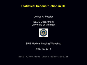
Regularization parameters: Dramatic effectsThibault et al., Med. Phys., Nov. 2007“q generalized gaussian” potential function with tuning parameters: β, δ, p, q:p1 t 2β ψ(t) β1 t/δ p qp q 211.1noise:(#lp/cm): 4.2p 2, q 1.2, δ 10 HUp q 1.110.97.210.88.236
Summary thus far1. Object parameterization2. System physical model3. Measurement statistical model4. Cost function: data-mismatch / regularization / constraintsReconstruction Method , Models Cost Function Algorithm5. Minimization algorithms:x̂x arg min Ψ(xx)x37
Choice 5: Minimization algorithms Conjugate gradients Converges slowly for CT Difficult to precondition due to weighting and regularization Difficult to enforce nonnegativity constraint Very easily parallelized Ordered subsets Initially converges faster than CG if many subsets used Does not converge without relaxation etc., but those slow it down Computes regularizer gradient R(xx) for every subset - expensive? Easily enforces nonnegativity constraint Easily parallelized Coordinate descent(Sauer and Bouman, T-SP, 1993) Converges high spatial frequencies rapidly, but low frequencies slowly Easily enforces nonnegativity constraint Challenging to parallelize Block coordinate descent(Benson et al., NSS/MIC, 2010) Spatial frequency convergence properties depend. Easily enforces nonnegativity constraint More opportunity to parallelize than CD38
Convergence rates(De Man et al., NSS/MIC 2005)In terms of iterations: CD OS CG Convergent OSIn terms of compute time? (it depends.)39
Ordered subsets convergenceTheoretically OS does not converge, but it may get “close enough,” evenwith regularization.CD200 iterOS41 subsets200 iterdifference0 10HUdisplay: 930 HU 58 HU(De Man et al., NSS/MIC 2005)Ongoing saga.(SPIE, ISBI, Fully 3D, .) 40
Example(movie)82-subset OS with two different (but similar) edge-preserving regularizers.One frame per every 10th iteration.41
Resolution characterization challengeOrig:RestoredimageusingPWLSδ 1:Noiselessblurryimage:1248normalized profile10 50horizontal location5Shape of edge response depends on contrast for edge-preserving regularizers.42
Assessing image quality Several talks in Session 4 Poster 7961-115, Rongping Zeng, Kyle J. MyersTask-based comparative study on iterative image reconstruction methodsfor limited-angle x-ray tomography Poster 7961-113, Pascal Theriault Lauzier, Jie Tang, Guang-Hong ChenQuantitative evaluation method of noise texture for iterativelyreconstructed x-ray CT images .Very important to be specific about which statistical reconstruction methodis being evaluated because results may vary significantly for different choicesof models, parameters, stopping rules, . What does “MTF” mean for nonlinear, shift-variant systems? “Less dose reduction for larger patients” “Resolution degrades as dose decreases”43
Some open problems Modeling Statistical modeling for very low-dose CT Resolution effects Spectral CT Object motion Parameter selection / performance characterization Performance prediction for nonquadratic regularization Effect of nonquadratic regularization on detection tasks Choice of regularization parameters for nonquadratic regularization Algorithms optimization algorithm design software/hardware implementation Moore’s law alone will not suffice(dual energy, dual source, motion, dynamic, smaller voxels .) Clinical evaluation .44
“Statistical” methods: Image domain Denoising methods sinogram y FBP noisy reconstruction xx iterative denoiser final image xˆ Remarkable advances in denoising methods in last decade Zhu & Milanfar, T-IP, Dec. 2010, using “steering ker