Transcription
Chapter 11Nonlinear Optimization ExamplesChapter Table of ContentsOVERVIEW . . . . . . . . . . . . . . . . . . . . . . . . . . . . . . . . . . . 297GETTING STARTED . . . . . . . . . . . . . . . . . . . . . . . . . . . . . . 299DETAILS . . . . . . . . . . . . . . . . . . . . . .Global Versus Local Optima . . . . . . . . . . .Kuhn-Tucker Conditions . . . . . . . . . . . . .Definition of Return Codes . . . . . . . . . . . .Objective Function and Derivatives . . . . . . . .Finite Difference Approximations of DerivativesParameter Constraints . . . . . . . . . . . . . . .Options Vector . . . . . . . . . . . . . . . . . .Termination Criteria . . . . . . . . . . . . . . .Control Parameters Vector . . . . . . . . . . . .Printing the Optimization History . . . . . . . .307307308309309314317319325332334NONLINEAR OPTIMIZATION EXAMPLES . . . . . . . .Example 11.1 Chemical Equilibrium . . . . . . . . . . . . . .Example 11.2 Network Flow and Delay . . . . . . . . . . . .Example 11.3 Compartmental Analysis . . . . . . . . . . . .Example 11.4 MLEs for Two-Parameter Weibull Distribution .Example 11.5 Profile-Likelihood-Based Confidence Intervals .Example 11.6 Survival Curve for Interval Censored Data . . .Example 11.7 A Two-Equation Maximum Likelihood ProblemExample 11.8 Time-Optimal Heat Conduction . . . . . . . . .336336340343353355357363367REFERENCES . . . . . . . . . . . . . . . . . . . . . . . . . . . . . . . . . . 371
296 Chapter 11. Nonlinear Optimization ExamplesSAS OnlineDoc : Version 8
Chapter 11Nonlinear Optimization ExamplesOverviewThe IML procedure offers a set of optimization subroutines for minimizing or maximizing a continuous nonlinear function f f (x) of n parameters, where x (x1 ; : : : ; xn )T . The parameters can be subject to boundary constraints and linearor nonlinear equality and inequality constraints. The following set of optimizationsubroutines is LPTRConjugate Gradient MethodDouble Dogleg MethodNelder-Mead Simplex MethodNewton-Raphson MethodNewton-Raphson Ridge Method(Dual) Quasi-Newton MethodQuadratic Optimization MethodTrust-Region MethodThe following subroutines are provided for solving nonlinear least-squares problems:NLPLMNLPHQNLevenberg-Marquardt Least-Squares MethodHybrid Quasi-Newton Least-Squares MethodsA least-squares problem is a special form of minimization problem where the objective function is defined as a sum of squares of other (nonlinear) functions.f (x) 12 ff12 (x) fm2 (x)gLeast-squares problems can usually be solved more efficiently by the least-squaressubroutines than by the other optimization subroutines.The following subroutines are provided for the related problems of computing finitedifference approximations for first- and second-order derivatives and of determininga feasible point subject to boundary and linear constraints:NLPFDDNLPFEAApproximate Derivatives by Finite DifferencesFeasible Point Subject to ConstraintsEach optimization subroutine works iteratively. If the parameters are subject onlyto linear constraints, all optimization and least-squares techniques are feasible-pointmethods; that is, they move from feasible point x(k) to a better feasible point x(k 1)by a step in the search direction s(k) , k 1; 2; 3; : : : . If you do not provide a feasiblestarting point x(0) , the optimization methods call the algorithm used in the NLPFEAsubroutine, which tries to compute a starting point that is feasible with respect to theboundary and linear constraints.
298 Chapter 11. Nonlinear Optimization ExamplesThe NLPNMS and NLPQN subroutines permit nonlinear constraints on parameters.For problems with nonlinear constraints, these subroutines do not use a feasiblepoint method; instead, the algorithms begin with whatever starting point you specify,whether feasible or infeasible.Each optimization technique requires a continuous objective function f f (x) andall optimization subroutines except the NLPNMS subroutine require continuous firstorder derivatives of the objective function f . If you do not provide the derivatives off , they are approximated by finite difference formulas. You can use the NLPFDDsubroutine to check the correctness of analytical derivative specifications.Most of the results obtained from the IML procedure optimization and least-squaressubroutines can also be obtained by using the NLP procedure in the SAS/OR product.The advantages of the IML procedure are as follows: You can use matrix algebra to specify the objective function, nonlinear constraints, and their derivatives in IML modules.The IML procedure offers several subroutines that can be used to specify theobjective function or nonlinear constraints, many of which would be very difficult to write for the NLP procedure.You can formulate your own termination criteria by using the "ptit" moduleargument.The advantages of the NLP procedure are as follows: Although identical optimization algorithms are used, the NLP procedure canbe much faster because of the interactive and more general nature of the IMLproduct.Analytic first- and second-order derivatives can be computed with a specialcompiler.Additional optimization methods are available in the NLP procedure that donot fit into the framework of this package.Data set processing is much easier than in the IML procedure. You can saveresults in output data sets and use them in following runs.The printed output contains more information.SAS OnlineDoc : Version 8
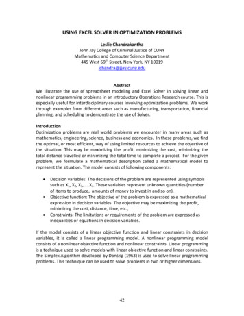
Getting Started 299Getting StartedUnconstrained Rosenbrock FunctionThe Rosenbrock function is defined asf (x) 12 f100(x2 , x21 )2 (1 , x1 )2 g 12 ff12 (x) f22 (x)g; x (x1 ; x2 )The minimum function value f f (x ) 0 is at the point x (1; 1).The following code calls the NLPTR subroutine to solve the optimization problem:proc iml;title ’Test of NLPTR subroutine: Gradient Specified’;start F ROSEN(x);y1 10. * (x[2] - x[1] * x[1]);y2 1. - x[1];f .5 * (y1 * y1 y2 * y2);return(f);finish F ROSEN;start G ROSEN(x);g j(1,2,0.);g[1] -200.*x[1]*(x[2]-x[1]*x[1]) - (1.-x[1]);g[2] 100.*(x[2]-x[1]*x[1]);return(g);finish G ROSEN;x {-1.2 1.};optn {0 2};call nlptr(rc,xres,"F ROSEN",x,optn) grd "G ROSEN";quit;The NLPTR is a trust-region optimization method. The F– ROSEN module represents the Rosenbrock function, and the G– ROSEN module represents its gradient.Specifying the gradient can reduce the number of function calls by the optimizationsubroutine. The optimization begins at the initial point x (,1:2; 1). For moreinformation on the NLPTR subroutine and its arguments, see the section “NLPTRCall” on page 667. For details on the options vector, which is given by the OPTNvector in the preceding code, see the section “Options Vector” on page 319.A portion of the output produced by the NLPTR subroutine is shown in Figure 11.1on page 300.SAS OnlineDoc : Version 8
300 Chapter 11. Nonlinear Optimization ExamplesTrust Region OptimizationWithout Parameter ScalingCRP Jacobian Computed by Finite DifferencesParameter Estimates2Optimization StartActive ConstraintsMax Abs GradientElementIter0107.8Rest Func Actarts Calls 9261.74390Objective FunctionRadiusMax AbsObj Fun GradientChange -16 6.96E-10 1.977E-70 0.00314Optimization ResultsIterationsHessian CallsObjective nction CallsActive ConstraintsMax Abs GradientElementActual Over PredChange3201.9773384E-70ABSGCONV convergence criterion satisfied.Optimization ResultsParameter EstimatesN ParameterEstimateGradientObjectiveFunction1 X12 X21.0000001.0000000.000000198-0.000000105Value of Objective Function 1.312814E-16Figure 11.1.NLPTR Solution to the Rosenbrock ProblemSince f (x) 21 ff12 (x) f22 (x)g, you can also use least-squares techniques in thissituation. The following code calls the NLPLM subroutine to solve the problem. Theoutput is shown in Figure ? on page ?.proc iml;title ’Test of NLPLM subroutine: No Derivatives’;start F ROSEN(x);y j(1,2,0.);y[1] 10. * (x[2] - x[1] * x[1]);y[2] 1. - x[1];return(y);SAS OnlineDoc : Version 8
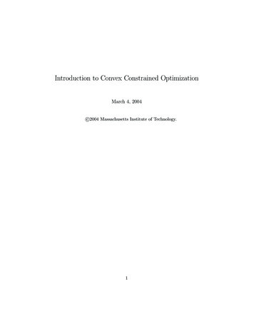
Getting Started 301finish F ROSEN;x {-1.2 1.};optn {2 2};call nlplm(rc,xres,"F ROSEN",x,optn);quit;The Levenberg-Marquardt least-squares method, which is the method used by theNLPLM subroutine, is a modification of the trust-region method for nonlinear leastsquares problems. The F– ROSEN module represents the Rosenbrock function. Notethat for least-squares problems, the m functions f1 (x); : : : ; fm (x) are specified aselements of a vector; this is different from the manner in which f (x) is specifiedfor the other optimization techniques. No derivatives are specified in the precedingcode, so the NLPLM subroutine computes finite difference approximations. For moreinformation on the NLPLM subroutine, see the section “NLPLM Call” on page 645.Constrained Betts FunctionThe linearly constrained Betts function (Hock & Schittkowski 1981) is defined asf (x) 0:01x21 x22 , 100with boundary constraints2 x1 50,50 x2 50and linear constraint10x1 , x2 10The following code calls the NLPCG subroutine to solve the optimization problem.The infeasible initial point x0 (,1; ,1) is specified, and a portion of the output isshown in Figure 11.2.proc iml;title ’Test of NLPCG subroutine: No Derivatives’;start F BETTS(x);f .01 * x[1] * x[1] x[2] * x[2] - 100.;return(f);finish F BETTS;con {2. -50. .,50. 50. .,10. -1. 1. 10.};x {-1. -1.};optn {0 2};call nlpcg(rc,xres,"F BETTS",x,optn,con);quit;SAS OnlineDoc : Version 8
302 Chapter 11. Nonlinear Optimization ExamplesThe NLPCG subroutine performs conjugate gradient optimization. It requires onlyfunction and gradient calls. The F– BETTS module represents the Betts function,and since no module is defined to specify the gradient, first-order derivatives arecomputed by finite difference approximations. For more information on the NLPCGsubroutine, see the section “NLPCG Call” on page 634. For details on the constraintmatrix, which is represented by the CON matrix in the preceding code, see the section“Parameter Constraints” on page 317.NOTE: Initial point was changed to be feasible for boundary andlinear constraints.Optimization StartParameter EstimatesGradientObjectiveEstimateFunctionN Parameter1 X12 0000002.000000-50.000000Optimization StartParameter ue of Objective Function -98.5376Linear Constraints159.00000 :10.0000 10.0000 * X1-Conjugate-Gradient OptimizationAutomatic Restart Update (Powell, 1977; Beale, 1972)Gradient Computed by Finite DifferencesParameter EstimatesLower BoundsUpper BoundsLinear ConstraintsFigure 11.2.SAS OnlineDoc : Version 82221NLPCG Solution to Betts Problem1.0000 * X2
Getting Started 303Optimization StartActive ConstraintsMax Abs GradientElementIter02Rest Func Actarts Calls Con123012379ObjectiveFunction011Objective Function-98.5376Max AbsObj Fun GradientChange Element-99.546821.0092-99.960000.4132-99.96000 2 -4.01834.985 -0.01820.500 -74E-7Optimization ResultsIterationsGradient CallsObjective FunctionSlope of SearchDirection39-99.96Function CallsActive ConstraintsMax Abs GradientElement1010-7.398365E-6ABSGCONV convergence criterion satisfied.Optimization ResultsParameter EstimatesGradientObjectiveEstimateFunctionN Parameter1 X12 ntLower BCValue of Objective Function -99.96Linear Constraints Evaluated at Solution[1]10.00000Figure 11.2. -10.0000 10.0000 * X1-1.0000 * X2(continued)Since the initial point (,1; ,1) is infeasible, the subroutine first computes a feasiblestarting point. Convergence is achieved after three iterations, and the optimal point isgiven to be x (2; 0) with an optimal function value of f f (x ) ,99:96. Formore information on the printed output, see the section “Printing the OptimizationHistory” on page 334.Rosen-Suzuki ProblemThe Rosen-Suzuki problem is a function of four variables with three nonlinear constraints on the variables. It is taken from Problem 43 of Hock and Schittkowski(1981). The objective function isf (x) x21 x22 2x23 x24 , 5x1 , 5x2 , 21x3 7x4SAS OnlineDoc : Version 8
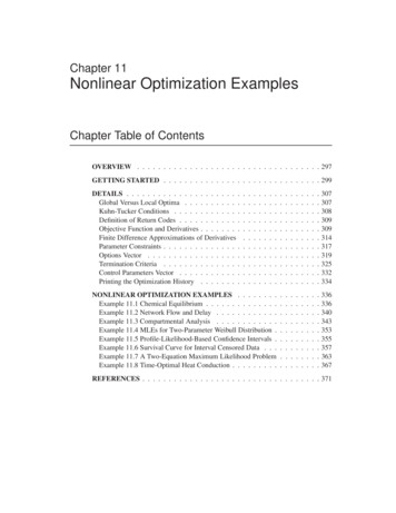
304 Chapter 11. Nonlinear Optimization ExamplesThe nonlinear constraints are0 8 , x21 , x22 , x23 , x24 , x1 x2 , x3 x40 10 , x21 , 2x22 , x23 , 2x24 x1 x40 5 , 2x21 , x22 , x23 , 2x1 x2 x4Since this problem has nonlinear constraints, only the NLPQN and NLPNMS subroutines are available to perform the optimization. The following code solves theproblem with the NLPQN subroutine:proc iml;start F HS43(x);f x*x‘ x[3]*x[3] - 5*(x[1] x[2]) - 21*x[3] 7*x[4];return(f);finish F HS43;start C HS43(x);c j(3,1,0.);c[1] 8 - x*x‘ - x[1] x[2] - x[3] x[4];c[2] 10 - x*x‘ - x[2]*x[2] - x[4]*x[4] x[1] x[4];c[3] 5 - 2.*x[1]*x[1] - x[2]*x[2] - x[3]*x[3]- 2.*x[1] x[2] x[4];return(c);finish C HS43;x j(1,4,1);optn j(1,11,.); optn[2] 3; optn[10] 3; optn[11] 0;call nlpqn(rc,xres,"F HS43",x,optn) nlc "C HS43";The F– HS43 module specifies the objective function, and the C– HS43 module specifies the nonlinear constraints. The OPTN vector is passed to the subroutine as the optinput argument. See the section “Options Vector” on page 319 for more information.The value of OPTN[10] represents the total number of nonlinear constraints, and thevalue of OPTN[11] represents the number of equality constraints. In the precedingcode, OPTN[10] 3 and OPTN[11] 0, which indicate that there are three constraints,all of which are inequality constraints. In the subroutine calls, instead of separatingmissing input arguments with commas, you can specify optional arguments with keywords, as in the CALL NLPQN statement in the preceding code. For details on theCALL NLPQN statement, see the section “NLPQN Call” on page 658.The initial point for the optimization procedure is x (1; 1; 1; 1), and the optimalpoint is x (0; 1; 2; ,1), with an optimal function value of f (x ) ,44. Part ofthe output produced is shown in Figure 11.3 on page 305.SAS OnlineDoc : Version 8
Getting Started 305Dual Quasi-Newton OptimizationModified VMCWD Algorithm of Powell (1978, 1982)Dual Broyden - Fletcher - Goldfarb - Shanno Update (DBFGS)Lagrange Multiplier Update of Powell(1982)Gradient Computed by Finite DifferencesJacobian Nonlinear Constraints Computed by Finite DifferencesParameter EstimatesNonlinear Constraints43Optimization StartObjective FunctionMaximum Gradient ofthe Lagran 08667-44.00011-44.00001-44.00000Figure 11.3.Maximum ConstraintViolationMaximumConstraint PredictedViola- Functiontion 097E-7MaximumGradElementof theStep LagranSizeFunc1.0005.6471.0005.0411.0001.0611.000 0.02971.000 0.009061.000 0.002191.000 0.00022Solution to the Rosen-Suzuki Problem by the NLPQN SubroutineSAS OnlineDoc : Version 8
306 Chapter 11. Nonlinear Optimization ExamplesOptimization ResultsIterationsGradient CallsObjective Function79-44.00000026Maximum ProjectedGradientMaximum Gradient ofthe Lagran Func0.00022653410.00022158Function CallsActive ConstraintsMaximum ConstraintViolationValue LagrangeFunctionSlope of SearchDirection929.1176306E-8-44-5.097332E-7FCONV2 convergence criterion satisfied.WARNING: The point x is feasible only at the LCEPSILON 1E-7 range.Optimization ResultsParameter EstimatesGradientObjectiveEstimateFunctionN -0.000020681Value of Objective Function -44.00000026Value of Lagrange Function -44Figure 11.3.(continued)In addition to the standard iteration history, the NLPQN subroutine includes the following information for problems with nonlinear constraints: conmax is the maximum value of all constraint violations.pred is the value of the predicted function reduction used with the GTOL andFTOL2 termination criteria.alfa is the step sizeof the quasi-Newton step.lfgmax is the maximum element of the gradient of the Lagrange function.SAS OnlineDoc : Version 8
Global Versus Local Optima 307DetailsGlobal Versus Local OptimaAll the IML optimization algorithms converge toward local rather than global optima.The smallest local minimum of an objective function is called the global minimum,and the largest local maximum of an objective function is called the global maximum.Hence, the subroutines may occasionally fail to find the global optimum. Suppose1 (3x4 , 28x3 84x2 , 96x1 64) x2 , which hasyou have the function, f (x) 271112a local minimum at f (1; 0) 1 and a global minimum at the point f (4; 0) 0.The following statements use two calls of the NLPTR subroutine to minimize thepreceding function. The first call specifies the initial point xa (0:5; 1:5), andthe second call specifies the initial point xb (3; 1). The first call finds the localoptimum x (1; 0), and the second call finds the global optimum x (4; 0).proc iml;start F GLOBAL(x);f (3*x[1]**4-28*x[1]**3 84*x[1]**2-96*x[1] 64)/27 x[2]**2;return(f);finish F GLOBAL;xa {.5 1.5};xb {3 -1};optn {0 2};call nlptr(rca,xra,"F GLOBAL",xa,optn);call nlptr(rcb,xrb,"F GLOBAL",xb,optn);print xra xrb;One way to find out whether the objective function has more than one local optimumis to run various optimizations with a pattern of different starting points.For a more mathematical definition of optimality, refer to the Kuhn-Tucker theoremin standard optimization literature. Using a rather nonmathematical language, a localminimizer x satisfies the following conditions: There exists a small, feasible neighborhood of x that does not contain anypoint x with a smaller function value f (x) f (x ).The vector of first derivatives (gradient) g (x ) rf (x ) of the objectivefunction f (projected toward the feasible region) at the point x is zero.The matrix of second derivatives G(x ) r2 f (x ) (Hessian matrix) of theobjective function f (projected toward the feasible region) at the point x ispositive definite.A local maximizer has the largest value in a feasible neighborhood and a negativedefinite Hessian.The iterative optimization algorithm terminates at the point xt , which should be ina small neighborhood (in terms of a user-specified termination criterion) of a localoptimizer x . If the point xt is located on one or more active boundary or generalSAS OnlineDoc : Version 8
308 Chapter 11. Nonlinear Optimization Exampleslinear constraints, the local optimization conditions are valid only for the feasibleregion. That is, the projected gradient, Z T g (xt ), must be sufficiently smallthe projected Hessian, Z T G(xt )Z , must be positive definite for minimizationproblems or negative definite for maximization problemsIf there are n active constraints at the point xt , the nullspace Z has zero columnsand the projected Hessian has zero rows and columns. A matrix with zero rows andcolumns is considered positive as well as negative definite.Kuhn-Tucker ConditionsThe nonlinear programming (NLP) problem with one objective function f and mconstraint functions ci , which are continuously differentiable, is defined as follows:minimizef (x);ci(x) 0;ci(x) 0;x 2 Rn; subject toi 1; : : : ; mei me 1; : : : ; mIn the preceding notation, n is the dimension of the function f (x), and me is thenumber of equality constraints. The linear combination of objective and constraintfunctionsL(x; ) f (x) ,mXi 1 i ci (x)is the Lagrange function, and the coefficients i are the Lagrange multipliers.If the functions f and ci are twice differentiable, the point x is an isolated localminimizer of the NLP problem, if there exists a vector ( 1 ; : : : ; m ) that meetsthe following conditions: Kuhn-Tucker conditions Second-order conditionci (x ) 0;i 1; : : : ; me ci (x ) 0; i 0; i ci(x ) 0; i me 1; : : : ; mrxL(x ; ) 0Each nonzero vector y2 Rn withyT rxci (x ) 0i 1; : : : ; me ;and 8i 2 me 1; : : : ; m; i 0satisfiesyT r2xL(x ; )y 0In practice, you cannot expect that the constraint functions ci (x ) will vanish withinmachine precision, and determining the set of active constraints at the solution x may not be simple.SAS OnlineDoc : Version 8
Objective Function and Derivatives 309Definition of Return CodesThe return code, which is represented by the output parameter rc in the optimization subroutines, indicates the reason for optimization termination. A positive valueindicates successful termination, while a negative value indicates unsuccessful termination. Table 11.1 gives the reason for termination associated with each returncode.Table 11.1.rc12345678910-1-2-3-4-5-6-7-8-9-10Summary of Return CodesReason for Optimization TerminationABSTOL criterion satisfied (absolute F convergence)ABSFTOL criterion satisfied (absolute F convergence)ABSGTOL criterion satisfied (absolute G convergence)ABSXTOL criterion satisfied (absolute X convergence)FTOL criterion satisfied (relative F convergence)GTOL criterion satisfied (relative G convergence)XTOL criterion satisfied (relative X convergence)FTOL2 criterion satisfied (relative F convergence)GTOL2 criterion satisfied (relative G convergence)n linear independent constraints are active at xr and none of them could bereleased to improve the function valueobjective function cannot be evaluated at starting pointderivatives cannot be evaluated at starting pointobjective function cannot be evaluated during iterationderivatives cannot be evaluated during iterationoptimization subroutine cannot improve the function value (this is a verygeneral formulation and is used for various circumstances)there are problems in dealing with linearly dependent active constraints(changing the LCSING value in the par vector can be helpful)optimization process stepped outside the feasible region and the algorithmto return inside the feasible region was not successful (changing the LCEPSvalue in the par vector can be helpful)either the number of iterations or the number of function calls is larger thanthe prespecified values in the tc vector (MAXIT and MAXFU)this return code is temporarily not used (it is used in PROC NLP indicatingthat more CPU than a prespecified value was used)a feasible starting point cannot be computedObjective Function and DerivativesThe input argument fun refers to an IML module that specifies a function that returnsf , a vector of length m for least-squares subroutines or a scalar for other optimizationsubroutines. The returned f contains the values of the objective function (or the leastsquares functions) at the point x. Note that for least-squares problems, you mustspecify the number of function values, m, with the first element of the opt argumentto allocate memory for the return vector. All the modules that you can specify asinput arguments ("fun", "grd", "hes", "jac", "nlc", "jacnlc", and "ptit") allow only asingle input argument, x, which is the parameter vector. Using the GLOBAL clause,SAS OnlineDoc : Version 8
310 Chapter 11. Nonlinear Optimization Examplesyou can provide more input arguments for these modules. Refer to the middle of thesection, "Compartmental Analysis" for an example.All the optimization algorithms assume that f is continuous inside the feasible region.For nonlinearly constrained optimization, this is also required for points outside thefeasible region. Sometimes the objective function cannot be computed for all pointsof the specified feasible region; for example, the function specification may containthe SQRT or LOG function, which cannot be evaluated for negative arguments. Youmust make sure that the function and derivatives of the starting point can be evaluated.There are two ways to prevent large steps into infeasible regions of the parameterspace during the optimization process: The preferred way is to restrict the parameter space by introducing moreboundary and linear constraints. For example, the boundary constraintxj 1E,10 prevents infeasible evaluations of log(xj ). If the function module takes the square root or the log of an intermediate result, you can use nonlinear constraints to try to avoid infeasible function evaluations. However, thismay not ensure feasibility.Sometimes the preferred way is difficult to practice, in which case the functionmodule may return a missing value. This may force the optimization algorithmto reduce the step length or the radius of the feasible region.All the optimization techniques except the NLPNMS subroutine require continuousfirst-order derivatives of the objective function f . The NLPTR, NLPNRA, and NLPNRR techniques also require continuous second-order derivatives. If you do notprovide the derivatives with the IML modules "grd", "hes", or "jac", they are automatically approximated by finite difference formulas. Approximating first-orderderivatives by finite differences usually requires n additional calls of the functionmodule. Approximating second-order derivatives by finite differences using onlyfunction calls can be extremely computationally expensive. Hence, if you decideto use the NLPTR, NLPNRA, or NLPNRR subroutines, you should specify at leastanalytical first-order derivatives. Then, approximating second-order derivatives byfinite differences requires only n or 2n additional calls of the function and gradientmodules.For all input and output arguments, the subroutines assume that the number of parameters n corresponds to the number of columns. For example, x, the input argument to the modules, and g , the output argument returnedby the "grd" module, are row vectors with n entries, and G, the Hessian matrixreturned by the "hes" module, must be a symmetric n n matrix.the number of functions, m, corresponds to the number of rows. For example,the vector f returned by the "fun" module must be a column vector with mentries, and in least-squares problems, the Jacobian matrix J returned by the"jac" module must be an m n matrix.You can verify your analytical derivative specifications by computing finite difference approximations of the derivatives of f with the NLPFDD subroutine. For mostSAS OnlineDoc : Version 8
Objective Function and Derivatives 311applications, the finite difference approximations of the derivatives will be very precise. Occasionally, difficult objective functions and zero x coordinates will causeproblems. You can use the par argument to specify the number of accurate digits inthe evaluation of the objective function; this defines the step size h of the first- andsecond-order finite difference formulas. See the section “Finite Difference Approximations of Derivatives” on page 314.Note: For some difficult applications, the finite difference approximations of derivatives that are generated by default may not be precise enough to solve the optimizationor least-squares problem. In such cases, you may be able to specify better derivativeapproximations by using a better approximation formula. You can submit your ownfinite difference approximations using the IML modules "grd", "hes", "jac", or "jacnlc". See Example 11.3 on page 343 for an illustration.In many applications, calculations used in the computation of f can help computederivatives at the same point efficiently. You can save and reuse such calculations withthe GLOBAL clause. As with many other optimization packages, the subroutinesperform calls of the "grd", "hes", or "jac" modules only after a call of the "fun"module.The following statements specify modules for the function, gradient, and Hessianmatrix of the Rosenbrock problem:proc iml;start F ROSEN(x);y1 10. * (x[2] - x[1] * x[1]);y2 1. - x[1];f .5 * (y1 * y1 y2 * y2);return(f);finish F ROSEN;start G ROSEN(x);g j(1,2,0.);g[1] -200.*x[1]*(x[2]-x[1]*x[1]) - (1.-x[1]);g[2] 100.*(x[2]-x[1]*x[1]);return(g);finish G ROSEN;start H ROSEN(x);h j(2,2,0.);h[1,1] -200.*(x[2] - 3.*x[1]*x[1]) 1.;h[2,2] 100.;h[1,2] -200. * x[1];h[2,1] h[1,2];return(h);finish H ROSEN;The following statements specify a module for the Rosenbrock function when considered as a least-squares problem. They also specify the Jacobian matrix of theleast-squares functions.SAS OnlineDoc : Version 8
312 Chapter 11. Nonlinear Optimization Examplesproc iml;start F ROSEN(x);y j(1,2,0.);y[1] 10. * (x[2] - x[1] * x[1]);y[2] 1. - x[1];return(y);finish F ROSEN;start J ROSEN(x);jac j(2,2,0.);jac[1,1] -20. * x[1]; jac[1,2] 10.;jac[2,1] -1.;jac[2,2] 0.;return(jac);finish J ROSEN;Diagonal or Sparse Hessian MatricesIn the unconstrained or only boundary constrained case, the NLPNRA algorithm cantake advantage of diagonal or sparse Hessian matrices submitted by the "hes" module.If the Hessian matrix G of the objective function f has a large proportion of zeros, youmay save computer time and memory by specifying a sparse Hessian of dimensionnn 3 rather than a dense n n Hessian. Each of the nn rows (i; j; g) of the matrixreturned by the sparse Hessian module defines a nonzero element gij of the Hessianmatrix. The row and column location is given by i and j , and g gives the nonzerovalue. During the optimization process, only the values g can be changed in each callof the Hessian module "hes"; the sparsity structure (i; j ) must be kept the same. Thatmeans that some of the values g can be zero
ficult to write for the NLP procedure. You can formulate your own termination criteria by using the "ptit" module argument. The advantages of the NLP procedure are as follows: Although identical optimization algorithms are used, the NLP procedure can be much faster because of th