Transcription
Introduction to Convex Constrained OptimizationMarch 4, 2004c 2004Massachusetts Institute of Technology.1
1Overview Nonlinear Optimization Portfolio Optimization An Inventory Reliability Problem Further concepts for nonlinear optimization Convex Sets and Convex Functions Convex Optimization Pattern Classification Some Geometry Problems On the Geometry of Nonlinear Optimization Classification of Nonlinear Optimization Problems Solving Separable Convex Optimization via Linear Optimization Optimality Conditions for Nonlinear Optimization A Few Concluding Remarks2Nonlinear versus Linear OptimizationRecall the basic linear optimization model:2
cT xLP : minimizexs.t.aT1 x··. aTm x bm ,b1 ,x n .In this model, all constraints are linear equalities or inequalities, and theobjective function is a linear function. In contrast, a nonlinear optimizationproblem can have nonlinear functions in the constraints and/or the objectivefunction:N LP : minimizexf (x)s.t.g1 (x)··. 0, gm (x) 0,x n ,In this model, we have f (x) : n and gi (x) : n , i 1, . . . , m.Below we present several examples of nonlinear optimization models.3
3Portfolio OptimizationPortfolio optimization models are used throughout the financial investmentmanagement sector. These are nonlinear models that are used to determinethe composition of investment portfolios.Investors prefer higher annual rates of return on investing to lower annual rates of return. Furthermore, investors prefer lower risk to higher risk.Portfolio optimization seeks to optimally trade off risk and return in investing.We consider n assets, whose annual rates of return Ri are random variables, i 1, . . . , n. The expected annual return of asset i is µi , i 1, . . . , n,and so if we invest a fraction xi of our investment dollar in asset i, theexpected return of the portfolio is:n µi xi µT xi 1where of course the fractions xi must satisfy:n xi eT x 1.0i 1andx 0.(Here, e is the vector of ones, e (1, 1, . . . , 1)T .The covariance of the rates of return of assets i and j is given asQij COV(i, j) .We can think of the Qij values as forming a matrix Q, whereby the varianceof portfolio is then:n n i 1 j 1COV(i, j)xi xj n n Qij xi xj xT Qx.i 1 j 1It should be noted, by the way, that the matrix Q will always by SPD(symmetric positive-definite).4
The “risk” in the portfolio is the standard deviation of the portfolio: STDEV xT Qx ,and the “return” of the portfolio is the expected annual rate of return of theportfolio:RETURN µT x .Suppose that we would like to determine the fractional investment valuesx1 , . . . , xn in order to maximize the return of the portfolio, subject to meeting some pre-specified target risk level. For example, we might want toensure that the standard deviation of the portfolio is at most 13.0%. Wecan formulate the following nonlinear optimization model:MAXIMIZE:s.t.FSUM:ST. DEV.:RETURN µT xeT x 1 xT Qx NONNEGATIVITY: x 013.0.An alternative version of the basic portfolio optimization model is todetermine the fractional investment values x1 , . . . , xn in order to minimizethe risk of the portfolio, subject to meeting a pre-specified target expectedreturn level. For example, we might want to ensure that the expected returnof the portfolio is at least 16.0%. We can formulate the following nonlinearoptimization model: MINIMIZE:s.t.FSUM:STDEV EXP. RETURN:µT x 16.0xT Qxet x 1NONNEGATIVITY: x 0 .5
Variations of this type of model are used pervasively by asset management companies worldwide. Also, this model can be extended to yield theCAPM (Capital Asset Pricing Model). Finally, we point out the Nobel Prizein economics was awarded in 1990 to Merton Miller, William Sharpe, andHarry Markowitz for their work on portfolio theory and portfolio models(and the implications for asset pricing).4An Inventory Reliability ProblemA colleague recently came to me with the follow problem that arises inanalyzing inventory management problems:Given positive coefficients hi , βi , di , i 1, . . . , m, and δ 0, solve fors1 , . . . , sm :IM P : minimizess.t.m i 1m i 1hi sidi e βi sisi5 δ, 0,i 1, . . . , mFurther Concepts for Nonlinear OptimizationRecall the basic nonlinear optimization model:6
N LP : minimizexf (x)s.t.g1 (x)··. 0, gm (x) 0,x n ,where f (x) : n and gi (x) : n , i 1, . . . , m. The feasibleregion of N LP is the setF {x g1 (x) 0, . . . , gm (x) 0}The ball centered at x̄ with radius is the set:B( x, ) : {x x x }We have the following definitions of local/global, strict/non-strict minima/maxima.Definition 5.1 x F is a local minimum of N LP if there exists 0such that f (x) f (y) for all y B(x, ) F.Definition 5.2 x F is a global minimum of N LP if f (x) f (y) for ally F.Definition 5.3 x F is a strict local minimum of N LP if there exists 0 such that f (x) f (y) for all y B(x, ) F, y x.Definition 5.4 x F is a strict global minimum of N LP if f (x) f (y)for all y F, y x.7
FFigure 1: Illustration of local versus global optima.Definition 5.5 x F is a local maximum of N LP if there exists 0such that f (x) f (y) for all y B(x, ) F.Definition 5.6 x F is a global maximum of N LP if f (x) f (y) for ally F.Definition 5.7 x F is a strict local maximum of N LP if there exists 0 such that f (x) f (y) for all y B(x, ) F, y x.Definition 5.8 x F is a strict global maximum of N LP if f (x) f (y)for all y F, y x.The phenomenon of local versus global optima is illustrated in Figure 1.5.1Convex Sets and FunctionsConvex sets and convex functions play an extremely important role in thestudy of optimization models. We start with the definition of a convex set:Definition 5.9 A subset S n is a convex set ifx, y S λx (1 λ)y Sfor any λ [0, 1].8
Figure 2: Illustration of convex and non-convex sets.Figure 3: Illustration of the intersection of convex sets.Figure 2 shows a convex set and a non-convex set.Proposition 5.1 If S, T are convex sets, then S T is a convex set.This proposition is illustrated in Figure 3.Proposition 5.2 The intersection of any collection of convex sets is a convex set.We now turn our attention to convex functions, defined below.Definition 5.10 A function f (x) is a convex function iff (λx (1 λ)y) λf (x) (1 λ)f (y)for all x and y and for all λ [0, 1].9
Figure 4: Illustration of convex and strictly convex functions.Definition 5.11 A function f (x) is a strictly convex function iff (λx (1 λ)y) λf (x) (1 λ)f (y)for all x and y and for all λ (0, 1), y x.Figure 4 illustrates convex and strictly convex functions.Now consider the following optimization problem, where the feasible region is simply described as the set F:P : minimizex f (x)s.t.x FProposition 5.3 Suppose that F is a convex set, f : F is a convex is a global minimum of ffunction, and x is a local minimum of P . Then xover F.Proof: Suppose x̄ is not a global minimum, i.e., there exists y F forwhich f (y) f ( x (1 λ)y, which is a convex combinationx). Let y(λ) λ of x̄ and y for λ [0, 1] (and therefore, y(λ) F for λ [0, 1]). Note thaty(λ) x̄ as λ 1.10
From the convexity of f (·),x (1 λ)y) λf ( x) (1 λ)f ( x)f (y(λ)) f (λ x) (1 λ)f (y) λf ( x) f ( x) for all λ (0, 1), and so x isfor all λ (0, 1). Therefore, f (y(λ)) f ( not a local minimum, resulting in a contradiction.q.e.d.Some examples of convex functions of one variable are: f (x) ax b f (x) x2 bx c f (x) x f (x) ln(x) for x 0 f (x) 1xfor x 0 f (x) ex5.2Concave Functions and MaximizationThe “opposite” of a convex function is a concave function, defined below:Definition 5.12 A function f (x) is a concave function iff (λx (1 λ)y) λf (x) (1 λ)f (y)for all x and y and for all λ [0, 1].Definition 5.13 A function f (x) is a strictly concave function iff (λx (1 λ)y) λf (x) (1 λ)f (y)for all x and y and for all λ (0, 1), , y x.Figure 5 illustrates concave and strictly concave functions.Now consider the maximization problem P :11
Figure 5: Illustration of concave and strictly concave functions.P : maximizex f (x)s.t.x FProposition 5.4 Suppose that F is a convex set, f : F is a concave is a global maximum offunction, and x is a local maximum of P . Then xf over F.5.3Linear Functions, Convexity, and ConcavityProposition 5.5 A linear function f (x) aT x b is both convex andconcave.Proposition 5.6 If f (x) is both convex and concave, then f (x) is a linearfunction.These properties are illustrated in Figure 6.12
Figure 6: A linear function is convex and concave.5.4Convex OptimizationSuppose that f (x) is a convex function. The setSα : {x f (x) α}is the level set of f (x) at level α.Proposition 5.7 If f (x) is a convex function, then Sα is a convex set.This proposition is illustrated in Figure 7.Now consider the following optimization:CP : minimizexf (x)s.t.g1 (x). 0,gm (x) 0,Ax b,x n ,13
Figure 7: The level sets of a convex function are convex sets.CP is called a convex optimization problem if f (x), g1 (x), . . . , gm (x) areconvex functions.Proposition 5.8 The feasible region of CP is a convex set.Proof: From Proposition 5.7, each of the setsFi : {x gi (x) 0}is a convex set, for i 1, . . . , m. Also, the affine set {x Ax b} is easilyshown to be a convex set. And from Proposition 5.2,F : {x Ax b} ( mi 1 Fi )is a convex set.q.e.d.Notice therefore that in CP we are minimizing a convex function over aconvex set. Applying Proposition 5.3, we have:Corollary 5.1 Any local minimum of CP will be a global minimum of CP .14
This is a most important aspect of convex optimization problem.Remark 1 If we replace “min” by “max” in CP and if f (x) is a concavefunction while g1 (x), . . . , gm (x) are convex functions, then any local maximum of CP will be a global maximum of CP .5.5Further Properties of Convex FunctionsThe next two propositions present two very important aspects of convexfunctions, namely that nonnegative sums of convex functions are convexfunctions, and that a convex function of an affine transformation of thevariables is a convex function.Proposition 5.9 If f1 (x) and f2 (x) are convex functions, and a, b 0,thenf (x) : af1 (x) bf2 (x)is a convex function.Proposition 5.10 If f (x) is a convex function and x Ay b, theng(y) : f (Ay b)is a convex function.A function f (x) is twice differentiable at x x̄ if there exists a vector f ( x) (called thex) (called the gradient of f (·)) and a symmetric matrix H( Hessian of f (·)) for which:1 T H( x)(x x) Rx (x) x x (x x) 2f (x) f ( x) f ( x)T (x x)2where Rx (x) 0 as x x. The gradient vector is the vector of partial derivatives: f (x̄) f ( x) f ( x),., x1 xn15 t.
The Hessian matrix is the matrix of second partial derivatives:H(x̄)ij x) 2 f ( . xi xjThe next theorem presents a characterization of a convex function interms of its Hessian matrix. Recall that SPSD means symmetric and positivesemi-definite, and SPD means symmetric and positive-definite.Theorem 5.1 Suppose that f (x) is twice differentiable on the open convexset S. Then f (x) is a convex function on the domain S if and only if H(x)is SPSD for all x S.The following functions are examples of convex functions in n-dimensions. f (x) aT x b f (x) 12 xT M x cT x where M is SPSD f (x) x for any norm · (see proof below) f (x) m i 1 ln(bi aTi x) for x satisfying Ax b.Corollary 5.2 If f (x) 12 xT M x cT x where M is a symmetric matrix,then f (·) is a convex function if and only if M is SPSD. Furthermore, f (·)is a strictly convex function if and only if M is SPD.Proposition 5.11 The norm function f (x) x is a convex function.Proof: Let f (x) : x . For any x, y and λ [0, 1], we have:f (λx (1 λ)y) λx (1 λ)y λx (1 λ)y λ x (1 λ) y 16
Figure 8: Illustration of a norm function. λf (x) (1 λ)f (y).q.e.d.This proposition is illustrated in Figure 8.When a convex function is differentiable, it must satisfy the followingproperty, called the “gradient inequality”.Proposition 5.12 If f (·) is a differentiable convex function, then for anyx, y,f (y) f (x) f (x)T (y x) .Even when a convex function is not differentiable, it must satisfy thefollowing “subgradient” inequality.Proposition 5.13 If f (·) is a convex function, then for every x, there mustexist some vector s for whichf (y) f (x) sT (y x)for any y .The vector s in this proposition is called a subgradient of f (·) at thepoint x.17
6More Examples of Convex Optimization Problems6.1A Pattern Classification Training ProblemWe are given: points a1 , . . . , ak n that have property “P” points b1 , . . . , bm n that do not have property “P”We would like to use these k m points to develop a linear rule that canbe used to predict whether or not other points x might or might not haveproperty P. In particular, we seek a vector v and a scalar β for which: v T ai β for all i 1, . . . , k v T bi β for all i 1, . . . , mWe will then use v, β to predict whether or not any other point c hasproperty P or not. If we are given another vector c, we will declare whetherc has property P or not as follows: If v T c β, then we declare that c has property P. If v T c β, then we declare that c does not have property P.We therefore seek v, β that define the hyperplaneHv,β : {x v T x β}for which: v T ai β for all i 1, . . . , k v T bi β for all i 1, . . . , m18
Figure 9: Illustration of the pattern classification problem.This is illustrated in Figure 9.In addition, we would like the hyperplane Hv,β to be as far away fromthe points a1 , . . . , ak , b1 , . . . , bk as possible. Elementary analysis shows thatthe distance of the hyperplane Hv,β to any point ai is equal tov T ai β v and similarly the distance of the hyperplane Hv,β to any point bi is equal toβ v T bi. v If we normalize the vector v so that v 1, then the minimum distance ofthe hyperplane Hv,β to the points a1 , . . . , ak , b1 , . . . , bk is then:min{v T a1 β, . . . , v T ak β, β v T b1 , . . . , β v T bm }Therefore we would also like v and β to satisfy: v 1, and min{v T a1 β, . . . , v T ak β, β v T b1 , . . . , β v T bm } is maximized.This results in the following optimization problem:19
P CP : maximizev,β,δδs.t.v T ai β δ,i 1, . . . , kβ v T bi δ,i 1, . . . , m v 1,v n , β Now notice that as written, P CP is not a convex optimization problem,due to the presence of the constraint “ v 1.” However, if we perform thefollowing transformation of variables:x βv, α δδ v 1 x , which is thethen maximizing δ is the same as maximizing x same as minimizing x . Therefore we can write the equivalent problem:CP CP : minimizex,αs.t. x xT ai α 1,i 1, . . . , kα xT bi 1,i 1, . . . , mx n , α Here we see that CP CP is a convex problem. We can solve CP CP forxα1, β x and δ x to obtain the solution ofx, α, and substitute v x P RP .20
Figure 10: Illustration of the minimum norm problem.6.2The Minimum Norm ProblemGiven a vector c, we would like to find the closest point to c that also satisfiesthe linear inequalities Ax b.This problem is:M N P : minimizex x c s.t.Ax bx nThis problem is illustrated in Figure 10.6.3The Fermat-Weber ProblemWe are given m points c1 , . . . , cm n . We would like to determine thelocation of a distribution center at the point x n that minimizes the sumof the distances from x to each of the points c1 , . . . , cm n . This problemis illustrated in Figure 11. It has the following formulation:21
F W P : minimizexm i 1s.t. x ci x nNotice that F W P is a convex unconstrained problem.6.4The Ball Circumscription ProblemWe are given m points c1 , . . . , cm n . We would like to determine thelocation of a distribution center at the point x n that minimizes themaximum distance from x to any of the points c1 , . . . , cm n . This problem is illustrated in Figure 12. It has the following formulation:BCP : minimizex,δs.t.δ x ci δ,i 1, . . . , m,x nThis is a convex (constrained) optimization problem.6.5The Analytic Center ProblemGiven a system of linear inequalities Ax b, we would like to determine a“nicely” interior point xˆ that satisfies Aˆx b. Of course, we would like thepoint to be as interior as possible, in some mathematically meaningful way.As it turns out, the solution of the following problem has some remarkableproperties:22
Figure 11: Illustration of the Fermat-Weber problem.Figure 12: Illustration of the ball circumscription problem.23
Figure 13: Illustration of the analytic center problem.ACP : maximizexm i 1(b Ax)is.t.Ax b,x nThis problem is illustrated in Figure 13.Proposition 6.1 Suppose that x̂ solves the analytic center problem ACP .Then for each i, we have:(b Ax̂)i wheres ims i : max(b Ax)i .Ax bNotice that as stated, ACP is not a convex problem, but it is equivalentto:24
Figure 14: Illustration of the circumscribed ellipsoid problem.CACP : minimizexm i 1 ln((b Ax)i )s.t.Ax b,x nNow notice that CACP is a convex problem.6.6The Circumscribed Ellipsoid ProblemWe are given m points c1 , . . . , cm n . We would like to determine anellipsoid of minimum volume that contains each of the points c1 , . . . , cm n . This problem is illustrated in Figure 14.Before we show the formulation of this problem, first recall that an SPDmatrix R and a given point z can be used to define an ellipsoid in n :ER,z : {y (y z)T R(y z) 1}.25
Figure 15: Illustration of an ellipsoid.Figure 15 shows an illustration of an ellipsoid.1One can prove that the volume of ER,z is proportional to det(R 1 ) 2 .Our problem is:1M CP1 : minimize det(R 1 ) 2R, zs.t.ci ER,z , i 1, . . . , k,R is SPD.11Now minimizing det(R 1 ) 2 is the same as minimizing ln(det(R 1 ) 2 ),since the logarithm function is strictly increasing in its argument. Also,11ln(det(R 1 ) 2 ) ln(det(R))2and so our problem is equivalent to:M CP2 : minimize ln(det(R))R, zs.t.(ci z)T R(ci z) 1, i 1, . . . , kR is SPD .26
We now factor R M 2 where M is SPD (that is, M is a square root ofR), and now M CP becomes:M CP3 : minimize ln(det(M 2 ))M, zs.t.(ci z)T M T M (ci z) 1, i 1, . . . , k,M is SPD.which is the same as:M CP4 : minimize 2 ln(det(M ))M, zs.t. M (ci z) 1, i 1, . . . , k,M is SPD.Next substitute y M z to obtain:M CP5 : minimize 2 ln(det(M ))M, ys.t. M ci y 1, i 1, . . . , k,M is SPD.It turns out that this is convex problem in the variables M, y.We can recover R and z after solving M CP5 by substituting R M 2and z M 1 y.77.1Classification of Nonlinear Optimization ProblemsGeneral Nonlinear Problemmin or max f (x)s.t. gi (x) bi , i 1, . . . , m27
7.2Unconstrained Optimizationmin or max f (x)s.t.7.3x nLinearly Constrained Problemsmin or max f (x)s.t.7.47.5Ax bLinear OptimizationmincT xs.t.Ax bQuadratic Problemmin cT x 12 xT Qxs.t.Ax bThe objective function here is min7.6j 1cj xj n n j 1 k 1xj Qjk xk .Quadratically Constrained Quadratic ProblemcT x 12 xT Qxmins.t.7.7n aTi x 12 xT Qi x bi , i 1, . . . , mSeparable Problemn mins.t.n j 1j 1fj (x)gij (xj ) bi , i 1, . . . , m28
7.7.1Example of a separable problem minx2 2y 1 z 3x2 y 2 cos z 9s.t.sin x 3 y sin(z π) 18x 0, y 0, z 07.8Convex Problemmins.t.f (x)gi (x) bi , i 1, . . . , mAx bwhere f (x) is a convex function and g1 (x), . . . , gm (x) are convex functions, or:maxs.t.f (x)gi (x) bi , i 1, . . . , mAx bwhere f (x) is a concave function and g1 (x), . . . , gm (x) are convex functions.29
7.8.1Example of a convex problemminx2 eys.t.x2 y 2 64x y 9(x 10)2 (y)2 25x 0, y 08Solving Separable Convex Optimization via Linear OptimizationConsider the problemmin (x1 2)2 2x2 9x3s.t.3x1 2x2 5x3 77x1 5x2 x3 8x1 , x2 , x3 0This problem has:1. linear constraints2. a separable objective function z f1 (x1 ) f2 (x2 ) 9x33. a convex objective function (since f1 (·) and f2 (·) are convex functions)In this case, we can approximate f1 (·) and f2 (·) by piecewise-linear (PL)functions. Suppose we know that 0 x1 9 and 0 x2 9. Referring toFigure 16 and Figure 17, we see that we can approximate these functions asfollows:30
Figure 16: PL approximation of f1 (·).Figure 17: PL approximation of f2 (·).31
f1 (x1 ) (x1 2)2 4 x1a 5x1b 11x1cwherex1 x1a x1b x1cand:0 x1a 3,0 x1b 3,0 x1c 3 .Similarly,721f2 (x2 ) 2x2 1 x2a 18 x2b 149 x2c333wherex2 x2a x2b x2cand:0 x2a 3,0 x2b 3,0 x2c 3The linear optimization approximation then is:32
min 4 x1a 5x1b 11x1c 1 73 x2a 18 32 x2b 149 13 x2c 9x3s.t.3x1 2x2 5x3 77x1 5x2 x3 8x1 , x2 , x3 0x1a x1b x1c x1x2a x2b x2c x20 x1a 30 x1b 30 x1c 30 x2a 30 x2b 30 x2c 39On the Geometry of Nonlinear OptimizationFigures 18, 19, and 20 show three possible configurations of optimal solutionsof nonlinear optimization models. These figures illustrate that unlike linearoptimization, the optimal solution of a nonlinear optimization problem neednot be a “corner point” of F . The optimal solution may be on the boundaryor even in the interior of F . However, as all three figures show, the optimalsolution will be characterized by how the contours of f (·) are “aligned” withthe feasible region F .33
Figure 18: First example of the geometry of the solution of a nonlinearoptimization problem.Figure 19: Second example of the geometry of the solution of a nonlinearoptimization problem.Figure 20: Third example of the geometry of the solution of a nonlinearoptimization problem.34
10Optimality Conditions for Nonlinear OptimizationConsider the convex problem:(CP) : min f (x)s.t.gi (x) bi ,i 1, . . . , m .where f (x), gi (x) are convex functions.We have:Theorem 10.1 (Karush-Kuhn-Tucker Theorem) Suppose that f (x), g1 (x), . . . , gm (x)are all convex functions. Then under very mild conditions, x̄ solves (CP) ifand only if there exists ȳi 0, i 1, . . . , m, such thatm ȳi gi ( x) 0 (gradients line up)(i) f ( x) (ii)gi (x̄) bi 0i 1(iii) ȳi 0(iv)10.1(feasibility)(multipliers must be nonnegative)x)) 0.y i (bi gi ( (multipliers for nonbinding constraints are zero)The KKT Theorem generalizes linear optimization strongdualityLet us see how the KKT Theorem applies to linear optimization. Considerthe following linear optimization problem and its dual:(LP): min cT x(LD): maxaTi x bi , i 1, . . . , mm i 1 yi bim i 1y 035yi ai c
Now let us look at the KKT Theorem applied to this problem. TheKKT Theorem states that if x solves LP, then there exists y i , i 1, . . . , mfor which:m ȳi gi ( x) : c (i) f ( x) (ii)gi (x̄) bi : aTi x bi 0i 1m i 1ȳi ai 0 (gradients line up)( primal feasibility)(iii) ȳi 0(iv)x)) : y i (bi aTi x) 0.y i (bi gi ( (complementary slackness)Now notice that (ii) is primal feasibility of x̄, and (i) and (iii) togetherare dual feasibility of ȳ. Finally, (iv) is complementary slackness. Therefore,the KKT Theorem here states that x and y together must be primal feasibleand dual feasible, and must satisfy complementary slackness.36
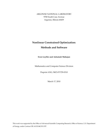
g1(x) 0 g1(x) f(x) f(x)–x g2(x)g3(x) 0g2(x) 0Figure 21: Illustration of the KKT Theorem.10.2Geometry of the KKT Theorem37
10.3An example of the KKT TheoremConsider the problem:min 6(x1 10)2 4(x2 12.5)2s.t.x21 (x2 5)2 50x21 3x22 200(x1 6)2 x22 37In this problem, we have:f (x) 6(x1 10)2 4(x2 12.5)2g1 (x) x21 (x2 5)2g2 (x) x21 3x22g3 (x) (x1 6)2 x22We also have: f (x) 12(x1 10) 8(x2 12.5) g1 (x) 2x1 2(x2 5) g2 (x) 2x16x238
g3 (x) 2(x1 6) 2x2Let us determine whether or not the point x ( x1 , x 2 ) (7, 6) is anoptimal solution to this problem.We first check for feasibility:g1 (x̄) 50 50 b1g2 (x̄) 157 200 b2g3 (x̄) 37 37 b3To check for optimality, we compute all gradients at x: f (x) 36 52 g1 (x) 14 2 g2 (x) 14 36 g3 (x) 2 12We next check to see if the gradients “line up”, by trying to solve fory1 0, y2 0, y3 0 in the following system:39
36 5214 y1 214 y2 362 0 y3 120Notice that y ( y1 , ȳ2 , ȳ3 ) (2, 0, 4) solves this system in nonnegativevalues, and that y2 0. Therefore x̄ is an optimal solution to this problem.10.4The KKT Theorem with Different formats of ConstraintsSuppose that our optimization problem is of the following form:(CPE) : min f (x)s.t.gi (x) bi ,i IaTi x bi ,i EThe KKT Theorem for this model is as follows:Theorem 10.2 (Karush-Kuhn-Tucker Theorem) Suppose that f (x), gi (x)are all convex functions for i I. Then under very mild conditions, x solves (CPE) if and only if there exists ȳi 0, i I and v̄i , i E such that(i) f ( x) i Iȳi gi ( x) k i Ev̄i ai 0 (gradients line up)(ii a) gi (x̄) bi 0, i I(feasibility)(ii b)ati x bi 0, i E(feasibility)(iii)ȳi 0, i I(nonnegative multipliers on inequalities)(iv)ȳi (bi gi (x̄)) 0, i I.(complementary slackness)What about the non-convex case? Let us consider a problem of thefollowing form:40
(NCE) : min f (x)gi (x) bi , i Is.t.hi (x) bi , i EWell, when the problem is not convex, we can at least assert that anyoptimal solution must satisfy the KKT conditions:Theorem 10.3 (Karush-Kuhn-Tucker Theorem) Under some very mild conditions, if x̄ solves (NCE), then there exists ȳi 0, i I and v̄i , i E suchthat f ( x) (i) i Iȳi gi ( x) i Ev̄i hi (x) 0 (gradients line up)(ii a) gi (x̄) bi 0, i I(feasibility)(ii b)hi (x) bi 0, i E(feasibility)(iii)ȳi 0(nonnegative multipliers on inequalities)(iv)ȳi (bi gi (x̄)) 0.(complementary slackness)11A Few Concluding Remarks1. Nonconvex optimization problems can be difficult to solve. This isbecause local optima may not be global optima. Most algorithms arebased on calculus, and so can only find a local optimum.2. Solution Methods. There are a large number of solution methods forsolving nonlinear constrained problems. Today, the most powerfulmethods fall into two classes: methods that try to generalize the simplex algorithm to the nonlinear case. methods that generalize the barrier method to the nonlinear case.41
3. Quadratic Problems. A quadratic problem is “almost linear”, andcan be solved by a special implementation of the simplex algorithm,called the complementary pivoting algorithm. Quadratic problems areroughly eight times harder to solve than linear optimization problemsof comparable size.42
3 Portfolio Optimization Portfolio optimization models are used throughout the financial investment management sector. These are nonlinear models that are used to determine the composition of investment portfolios. Investors prefer higher annual rates