Transcription
USING EXCEL SOLVER IN OPTIMIZATION PROBLEMSLeslie ChandrakanthaJohn Jay College of Criminal Justice of CUNYMathematics and Computer Science Department445 West 59th Street, New York, NY 10019lchandra@jjay.cuny.eduAbstractWe illustrate the use of spreadsheet modeling and Excel Solver in solving linear andnonlinear programming problems in an introductory Operations Research course. This isespecially useful for interdisciplinary courses involving optimization problems. We workthrough examples from different areas such as manufacturing, transportation, financialplanning, and scheduling to demonstrate the use of Solver.IntroductionOptimization problems are real world problems we encounter in many areas such asmathematics, engineering, science, business and economics. In these problems, we findthe optimal, or most efficient, way of using limited resources to achieve the objective ofthe situation. This may be maximizing the profit, minimizing the cost, minimizing thetotal distance travelled or minimizing the total time to complete a project. For the givenproblem, we formulate a mathematical description called a mathematical model torepresent the situation. The model consists of following components: Decision variables: The decisions of the problem are represented using symbolssuch as X1, X2, X3, .Xn. These variables represent unknown quantities (numberof items to produce, amounts of money to invest in and so on).Objective function: The objective of the problem is expressed as a mathematicalexpression in decision variables. The objective may be maximizing the profit,minimizing the cost, distance, time, etc.,Constraints: The limitations or requirements of the problem are expressed asinequalities or equations in decision variables.If the model consists of a linear objective function and linear constraints in decisionvariables, it is called a linear programming model. A nonlinear programming modelconsists of a nonlinear objective function and nonlinear constraints. Linear programmingis a technique used to solve models with linear objective function and linear constraints.The Simplex Algorithm developed by Dantzig (1963) is used to solve linear programmingproblems. This technique can be used to solve problems in two or higher dimensions.42
In this paper we show how to use spreadsheet modeling and Excel Solver for solvinglinear and nonlinear programming problems.Spreadsheet Modeling and Excel SolverA mathematical model implemented in a spreadsheet is called a spreadsheet model.Major spreadsheet packages come with a built-in optimization tool called Solver. Nowwe demonstrate how to use Excel spreadsheet modeling and Solver to find the optimalsolution of optimization problems.If the model has two variables, the graphical method can be used to solve the model.Very few real world problems involve only two variables. For problems with more thantwo variables, we need to use complex techniques and tedious calculations to find theoptimal solution. The spreadsheet and solver approach makes solving optimizationproblems a fairly simple task and it is more useful for students who do not have strongmathematics background.The first step is to organize the spreadsheet to represent the model. We use separatecells to represent decision variables, create a formula in a cell to represent the objectivefunction and create a formula in a cell for each constraint left hand side. Once themodel is implemented in a spreadsheet, next step is to use the Solver to find thesolution. In the Solver, we need to identify the locations (cells) of objective function,decision variables, nature of the objective function (maximize/minimize) andconstraints.Example One (Linear model): Investment ProblemOur first example illustrates how to allocate money to different bonds to maximize thetotal return (Ragsdale 2011, p. 121).A trust office at the Blacksburg National Bank needs to determine how to invest 100,000 in following collection of bonds to maximize the annual HighHighYesYesNoYesNoThe officer wants to invest at least 50% of the money in short term issues and no morethan 50% in high-risk issues. At least 30% of the funds should go in tax-free investments,and at least 40% of the total return should be tax free.Creating the Linear Programming model to represent the problem:Decision variables are the amounts of money should be invested in each bond.X1 Amount of money to invest in Bond A43
X2 Amount of money to invest in Bond BX3 Amount of money to invest in Bond CX4 Amount of money to invest in Bond DX5 Amount of money to invest in Bond EObjective Function:Objective is to maximize the total annual return.Maximize f(X1, X2, X3, X4, X5) 9.5%X1 8%X2 9%X3 9%X4 9%X5Constraints:Total investment:X1 X2 X3 X4 X5 100,000.At least 50% of the money goes to short term issues:X2 X5 50,000.No more than 50% of the money should go to high risk issues:X1 X4 X5 50,000.At least 30% of the money should go to tax free investments:X1 X2 X4 30,000.At least 40% of the total annual return should be tax free:9.5%X1 8%X2 9%X4 40%(9.5%X1 8%X2 9%X3 9%X4 9%X5)Nonnegativity constraints (all the variables should be nonnegative):X1, X2, X3, X4, X5 0.Complete linear programming model:Max: .095X1 .08X2 .09X3 .09X4 .09X5Subject to:X1 X2 X3 X4 X5 100,000.X2 X5 50,000.X1 X4 X5 50,000.X1 X2 X4 30,000.9.5%X1 8%X2 9%X4 40%(9.5%X1 8%X2 9%X3 9%X4 9%X5)X1, X2, X3, X4, X5 0.Spreadsheet model and Solver implementation:Implementing the problem in an Excel spreadsheet and Solver formulation produces thefollowing spreadsheet and Solver parameters. The cells B6 through B10 represent thefive decision variables. The cell C13 represents the objective function. The cells B11,E11, G11, I11, B14, and B15 represent the constraint left hand sides. The nonnegativityconstraint is not implemented in the spreadsheet and it can be implemented in theSolver. The complete set of constraints, target cell (objective function cell), variable cells(changing cells) and whether to maximize or minimize the objective function areidentified in the Solver parameters box.44
Figure 1: Spreadsheet implementation of example oneFigure 2: Solver implementation of example oneFigure 3: Spreadsheet with optimal solution of example one45
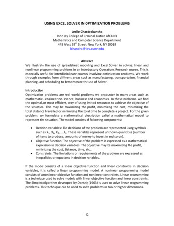
Optimal money allocation:Amount invested in Bond A X1 20, 339.Amount invested in Bond B X2 20, 339.Amount invested in Bond C X3 29, 661.Amount invested in Bond D X4 0.Amount invested in Bond E X5 29, 661.The Maximum annual return is 8,898.00Example Two (Nonlinear model): Network Flow ProblemThis example illustrates how to find the optimal path to transport hazardous material (Ragsdale, 2011, p.367)Safety Trans is a trucking company that specializes transporting extremely valuable andextremely hazardous materials. Due to the nature of the business, the company placesgreat importance on maintaining a clean driving safety record. This not only helps keeptheir reputation up but also helps keep their insurance premium down. The company isalso conscious of the fact that when carrying hazardous materials, the environmentalconsequences of even a minor accident could be disastrous.Safety Trans likes to ensure that it selects routes that are least likely to result in anaccident. The company is currently trying to identify the safest routes for carrying a loadof hazardous materials from Los Angeles to Amarillo, Texas. The following networksummarizes the routes under consideration. The numbers on each arc represent theprobability of having an accident on each potential leg of the journey.AlbuquerqueFlagstaff0.0010.006Las Vegas8620.001Amarillo0.003Los 40.0050.0020.002Phoenix9375San Diego0.0100.003TucsonLas CrucesFigure 4: Network diagram of example two460.003Lubbock
The objective is to find the route that minimizes the probability of having an accident, orequivalently, the route that maximizes the probability of not having an accident.Creating the mathematical model to represent the problem:Each decision variable indicates whether or not a particular route is taken (they areknown as binary variables). We will define these variables in following way:Xij 1 , if the route from node i to node j is selected, and Xij 0 otherwise.Let Pij be the probability of having an accident while travelling from node i to node j(1- Pij is the probability of not having an accident).Objective function:Minimize the probability of having an accident or equivalently, maximize the probabilityof not having an accident. Note that this objective function is nonlinear.Maximize f(X12, X13, .) (1-P12*X12) (1-P13*X13) (1 – P14*X14) (1 – P24*X24) . (1 P9.10*X9,10)Constraints:We use the following strategy to construct constraints: That is, supply one unit at thestarting node and demand one unit at the ending node, and for every other node,demand or supply is zero. We find the route in which the one unit travels.Total supply 1, and total demand 1, so for each node,Net flow (Inflow – Outflow) demand or supply for that node (Balance of flow rule).Then we have following set of constraints:Node 1: - X12 – X13 – X14 -1Node 2: X12 – X24 – X26 0Node 3: X13 – X34 – X35 0Node 4: X14 X24 X34 – X45 – X46 – X48 0Node 5: X35 X45 – X57 0Node 6: X26 X46 - X67 – X68 0Node 7: X57 X67 – X78 – X7,10 0Node 8: X48 X68 X78 – X8,10 0Node 9: X79 – X9,10 0Node 10: X7,10 X8,10 X 9,10 1Complete nonlinear Programming model:Maximize: (1-P12*X12) (1-P13*X13) (1 – P14*X14) (1 – P24*X24) . (1-P9.10*X9,10)Subject to:- X12 – X13 – X14 -1 X12 – X24 – X26 0 X13 – X34 – X35 047
X14 X24 X34 – X45 – X46 – X48 0 X35 X45 – X57 0 X26 X46 - X67 – X68 0 X57 X67 – X78 – X7,10 0 X48 X68 X78 – X8,10 0 X79 – X9,10 0 X7,10 X8,10 X 9,10 1All Xij are binary.Spreadsheet model and Solver implementation:Figure 5: Spreadsheet implementation of example TwoFigure 6: Solver implementation of example two48
Figure 7: Spreadsheet with optimal solution of example twoThe optimal path:The route that minimizes the probability of having an accident is given below:Los Angeles to PhoenixPhoenix to FlagstaffFlagstaff to AlbuquerqueAlbuquerque to Amarillo.Conclusion:Optimization problems in many fields can be modeled and solved using Excel Solver. Itdoes not require knowledge of complex mathematical concepts behind the solutionalgorithms. This way is particularly helpful for students who are non math majors andstill want to take theses courses.References:1) Cliff T. Ragsdale, 2011, Spreadsheet Modeling and Decision Analysis, 6th Edition.SOUTH-WESTERN, Cengage Learning.2) Dantzig, G. B. 1963, Linear Programming and Extensions, Princeton UniversityPress, Princeton, NJ.3) John Walkenbach, 2007, Excel 2007 Formulas, John Wiley and Sons.49
linear and nonlinear programming problems. Spreadsheet Modeling and Excel Solver A mathematical model implemented in a spreadsheet is called a spreadsheet model. Major spreadsheet packages come with a built-in optimization tool called Solver. Now we demonstrate how to use Excel