Transcription
PipingCalculationsManualE. Shashi Menon, P.E.SYSTEK Technologies, Inc.McGraw-HillNew York Chicago San Francisco Lisbon LondonMadrid Mexico City Milan New Delhi San JuanSeoul Singapore Sydney Toronto
Dedicated to my mother
ABOUT THE AUTHORE. SHASHI MENON, P.E., has over 29 years’ experience in theoil and gas industry, holding positions as design engineer,project engineer, engineering manager, and chief engineerfor major oil and gas companies in the United States. He isthe author of Liquid Pipeline Hydraulics and severaltechnical papers. He has taught engineering and computercourses, and is also developer and co-author of over a dozenPC software programs for the oil and gas industry.Mr. Menon lives in Lake Havasu City, Arizona.
PrefaceThis book covers piping calculations for liquids and gases in singlephase steady state flow for various industrial applications. Pipe sizingand capacity calculations are covered mainly with additional analysis ofstrength requirement for pipes. In each case the basic theory necessaryis presented first followed by several example problems fully worked outillustrating the concepts discussed in each chapter. Unlike a textbookor a handbook the focus is on solving actual practical problems that theengineer or technical professional may encounter in their daily work.The calculation manual approach has been found to be very successfuland I want to thank Ken McCombs of McGraw-Hill for suggesting thisformat.The book consists of ten chapters and three appendices. As far aspossible calculations are illustrated using both US Customary Systemof units as well as the metric or SI units. Piping calculations involvingwater are covered in the first three chapters titled Water Systems Piping, Fire Protection Piping Systems and Wastewater and StormwaterPiping. Water Systems Piping address transportation of water in shortand long distance pipelines. Pressure loss calculations, pumping horsepower required and pump analysis are discussed with numerous examples. The chapter on Fire Protection Piping Systems covers sprinklersystem design for residential and commercial buildings. WastewaterSystems chapter addresses how wastewater and stormwater pipingis designed. Open channel gravity flow in sewer lines are also discussed.Chapter 4 introduces the basics of steam piping systems. Flow of saturated and superheated steam through pipes and nozzles are discussedand concepts explained using example problems.Chapter 5 covers the flow of compressed air in piping systems including flow through nozzles and restrictions. Chapter 6 addresses transportation of oil and petroleum products through short and long distancepipelines. Various pressure drop equations used in the oil industry arexv
xviPrefacereviewed using practical examples. Series and parallel piping configurations are analyzed along with pumping requirements and pumpperformance. Economic analysis is used to compare alternatives for expanding pipeline throughput.Chapter 7 covers transportation of natural gas and other compressible fluids through pipeline. Calculations illustrate how gas piping aresized, pressures required and how compressor stations are located onlong distance gas pipelines. Economic analysis of pipe loops versus compression for expanding throughput are discussed. Fuel Gas DistributionPiping System is covered in chapter 8. In this chapter low pressure gaspiping are analyzed with examples involving Compressed Natural Gas(CNG) and Liquefied Petroleum Gas (LPG).Chapter 9 covers Cryogenic and Refrigeration Systems Piping. Commonly used cryogenic fluids are reviewed and capacity and pipe sizingillustrated. Since two phase flow may occur in some cryogenic pipingsystems, the Lockhart and Martinelli correlation method is used in explaining flow of cryogenic fluids. A typical compression refrigerationcycle is explained and pipe sizing illustrated for the suction and discharge lines.Finally, chapter 10 discusses transportation of slurry and sludge systems through pipelines. Both newtonian and nonnewtonian slurry systems are discussed along with different Bingham and pseudo-plasticslurries and their behavior in pipe flow. Homogenous and heterogeneous flow are covered in addition to pressure drop calculations inslurry pipelines.I would like to thank Ken McCombs of McGraw-Hill for suggestingthe subject matter and format for the book and working with me onfinalizing the contents. He was also aggressive in followthrough to getthe manuscript completed within the agreed time period. I enjoyedworking with him and hope to work on another project with McGrawHill in the near future. Lucy Mullins did most of the copyediting. Shewas very meticulous and thorough in her work and I learned a lot fromher about editing technical books. Ben Kolstad, Editorial Services Manager of International Typesetting and Composition (ITC), coordinatedthe work wonderfully. Neha Rathor and her team at ITC did the typesetting. I found ITC’s work to be very prompt, professional, and of highquality.Needless to say, I received a lot of help during the preparation ofthe manuscript. In particular I want to thank my wife Pramila forthe many hours she spent on the computer typing the manuscript andmeticulously proof reading to create the final work product. My fatherin-law, A. Mukundan, a retired engineer and consultant, also provided
Prefacexviivaluable guidance and help in proofing the manuscript. Finally, I wouldlike to dedicate this book to my mother, who passed away recently, butshe definitely was aware of my upcoming book and provided her usualencouragement throughout my effort.E. Shashi Menon
ContentsPrefacexvChapter 1. Water Systems PipingIntroduction1.1 Properties of Water1.1.1 Mass and Weight1.1.2 Density and Specific Weight1.1.3 Specific Gravity1.1.4 Viscosity1.2 Pressure1.3 Velocity1.4 Reynolds Number1.5 Types of Flow1.6 Pressure Drop Due to Friction1.6.1 Bernoulli’s Equation1.6.2 Darcy Equation1.6.3 Colebrook-White Equation1.6.4 Moody Diagram1.6.5 Hazen-Williams Equation1.6.6 Manning Equation1.7 Minor Losses1.7.1 Valves and Fittings1.7.2 Pipe Enlargement and Reduction1.7.3 Pipe Entrance and Exit Losses1.8 Complex Piping Systems1.8.1 Series Piping1.8.2 Parallel Piping1.9 Total Pressure Required1.9.1 Effect of Elevation1.9.2 Tight Line Operation1.9.3 Slack Line Flow1.10 Hydraulic Gradient1.11 Gravity Flow1.12 Pumping 41424445454750vii
viiiContents1.13 Pumps1.13.1 Positive Displacement Pumps1.13.2 Centrifugal Pumps1.13.3 Pumps in Series and Parallel1.13.4 System Head Curve1.13.5 Pump Curve versus System Head Curve1.14 Flow Injections and Deliveries1.15 Valves and Fittings1.16 Pipe Stress Analysis1.17 Pipeline EconomicsChapter 2. Fire Protection Piping SystemsIntroduction2.1 Fire Protection Codes and Standards2.2 Types of Fire Protection Piping2.2.1 Belowground Piping2.2.2 Aboveground Piping2.2.3 Hydrants and Sprinklers2.3 Design of Piping System2.3.1 Pressure2.3.2 Velocity2.4 Pressure Drop Due to Friction2.4.1 Reynolds Number2.4.2 Types of Flow2.4.3 Darcy-Weisbach Equation2.4.4 Moody Diagram2.4.5 Hazen-Williams Equation2.4.6 Friction Loss Tables2.4.7 Losses in Valves and Fittings2.4.8 Complex Piping Systems2.5 Pipe Materials2.6 Pumps2.6.1 Centrifugal Pumps2.6.2 Net Positive Suction Head2.6.3 System Head Curve2.6.4 Pump Curve versus System Head Curve2.7 Sprinkler System DesignChapter 3. Wastewater and Stormwater PipingIntroduction3.1 Properties of Wastewater and Stormwater3.1.1 Mass and Weight3.1.2 Density and Specific Weight3.1.3 Volume3.1.4 Specific Gravity3.1.5 Viscosity3.2 Pressure3.3 Velocity3.4 Reynolds Number3.5 Types of 133133134134136138140141
Contents3.6 Pressure Drop Due to Friction3.6.1 Manning Equation3.6.2 Darcy Equation3.6.3 Colebrook-White Equation3.6.4 Moody Diagram3.6.5 Hazen-Williams Equation3.7 Minor Losses3.7.1 Valves and Fittings3.7.2 Pipe Enlargement and Reduction3.7.3 Pipe Entrance and Exit Losses3.8 Sewer Piping Systems3.9 Sanitary Sewer System Design3.10 Self-Cleansing Velocity3.11 Storm Sewer Design3.11.1 Time of Concentration3.11.2 Runoff Rate3.12 Complex Piping Systems3.12.1 Series Piping3.12.2 Parallel Piping3.13 Total Pressure Required3.13.1 Effect of Elevation3.13.2 Tight Line Operation3.13.3 Slack Line Flow3.14 Hydraulic Gradient3.15 Gravity Flow3.16 Pumping Horsepower3.17 Pumps3.17.1 Positive Displacement Pumps3.17.2 Centrifugal Pumps3.18 Pipe Materials3.19 Loads on Sewer PipeChapter 4. Steam Systems PipingIntroduction4.1 Codes and Standards4.2 Types of Steam Systems Piping4.3 Properties of Steam4.3.1 Enthalpy4.3.2 Specific Heat4.3.3 Pressure4.3.4 Steam Tables4.3.5 Superheated Steam4.3.6 Volume4.3.7 Viscosity4.4 Pipe Materials4.5 Velocity of Steam Flow in Pipes4.6 Pressure Drop4.6.1 Darcy Equation for Pressure Drop4.6.2 Colebrook-White Equation4.6.3 Unwin 229231
xContents4.6.4 Babcock Formula4.6.5 Fritzche’s EquationNozzles and OrificesPipe Wall ThicknessDetermining Pipe SizeValves and Fittings4.10.1 Minor Losses4.10.2 Pipe Enlargement and Reduction4.10.3 Pipe Entrance and Exit Losses232233237245246247248249251Chapter 5. Compressed-Air Systems Piping2534.74.84.94.10Introduction5.1 Properties of Air5.1.1 Relative Humidity5.1.2 Humidity Ratio5.2 Fans, Blowers, and Compressors5.3 Flow of Compressed Air5.3.1 Free Air, Standard Air, and Actual Air5.3.2 Isothermal Flow5.3.3 Adiabatic Flow5.3.4 Isentropic Flow5.4 Pressure Drop in Piping5.4.1 Darcy Equation5.4.2 Churchill Equation5.4.3 Swamee-Jain Equation5.4.4 Harris Formula5.4.5 Fritzsche Formula5.4.6 Unwin Formula5.4.7 Spitzglass Formula5.4.8 Weymouth Formula5.5 Minor Losses5.6 Flow of Air through Nozzles5.6.1 Flow through a RestrictionChapter 6. Oil Systems ionDensity, Specific Weight, and Specific GravitySpecific Gravity of Blended ProductsViscosityViscosity of Blended ProductsBulk ModulusVapor PressurePressureVelocityReynolds NumberTypes of FlowPressure Drop Due to Friction6.11.1 Bernoulli’s Equation6.11.2 Darcy 0322325326327327329
Contents6.126.136.146.156.166.176.186.196.206.11.3 Colebrook-White Equation6.11.4 Moody Diagram6.11.5 Hazen-Williams Equation6.11.6 Miller Equation6.11.7 Shell-MIT Equation6.11.8 Other Pressure Drop EquationsMinor Losses6.12.1 Valves and Fittings6.12.2 Pipe Enlargement and Reduction6.12.3 Pipe Entrance and Exit LossesComplex Piping Systems6.13.1 Series Piping6.13.2 Parallel PipingTotal Pressure Required6.14.1 Effect of Elevation6.14.2 Tight Line OperationHydraulic GradientPumping HorsepowerPumps6.17.1 Positive Displacement Pumps6.17.2 Centrifugal Pumps6.17.3 Net Positive Suction Head6.17.4 Specific Speed6.17.5 Effect of Viscosity and Gravity on Pump PerformanceValves and FittingsPipe Stress AnalysisPipeline EconomicsChapter 7. Gas Systems PipingIntroduction7.1 Gas Properties7.1.1 Mass7.1.2 Volume7.1.3 Density7.1.4 Specific Gravity7.1.5 Viscosity7.1.6 Ideal Gases7.1.7 Real Gases7.1.8 Natural Gas Mixtures7.1.9 Compressibility Factor7.1.10 Heating Value7.1.11 Calculating Properties of Gas Mixtures7.2 Pressure Drop Due to Friction7.2.1 Velocity7.2.2 Reynolds Number7.2.3 Pressure Drop Equations7.2.4 Transmission Factor and Friction Factor7.3 Line Pack in Gas Pipeline7.4 Pipes in Series7.5 Pipes in Parallel7.6 Looping 33435439447
xiiContents7.7 Gas Compressors7.7.1 Isothermal Compression7.7.2 Adiabatic Compression7.7.3 Discharge Temperature of Compressed Gas7.7.4 Compressor Horsepower7.8 Pipe Stress Analysis7.9 Pipeline EconomicsChapter 8. Fuel Gas Distribution Piping SystemsIntroductionCodes and StandardsTypes of Fuel GasGas PropertiesFuel Gas System PressuresFuel Gas System ComponentsFuel Gas Pipe SizingPipe MaterialsPressure TestingLPG Transportation8.9.1 Velocity8.9.2 Reynolds Number8.9.3 Types of Flow8.9.4 Pressure Drop Due to Friction8.9.5 Darcy Equation8.9.6 Colebrook-White Equation8.9.7 Moody Diagram8.9.8 Minor Losses8.9.9 Valves and Fittings8.9.10 Pipe Enlargement and Reduction8.9.11 Pipe Entrance and Exit Losses8.9.12 Total Pressure Required8.9.13 Effect of Elevation8.9.14 Pump Stations Required8.9.15 Tight Line Operation8.9.16 Hydraulic Gradient8.9.17 Pumping Horsepower8.10 LPG Storage8.11 LPG Tank and Pipe Sizing8.18.28.38.48.58.68.78.88.9Chapter 9. Cryogenic and Refrigeration Systems PipingIntroduction9.1 Codes and Standards9.2 Cryogenic Fluids and Refrigerants9.3 Pressure Drop and Pipe Sizing9.3.1 Single-Phase Liquid Flow9.3.2 Single-Phase Gas Flow9.3.3 Two-Phase Flow9.3.4 Refrigeration Piping9.4 Piping 02503506506508510511519519520520523523552578584598
ContentsChapter 10. Slurry and Sludge Systems PipingIntroduction10.1 Physical Properties10.2 Newtonian and Nonnewtonian Fluids10.2.1 Bingham Plastic Fluids10.2.2 Pseudo-Plastic Fluids10.2.3 Yield Pseudo-Plastic Fluids10.3 Flow of Newtonian Fluids10.4 Flow of Nonnewtonian Fluids10.4.1 Laminar Flow of Nonnewtonian Fluids10.4.2 Turbulent Flow of Nonnewtonian Fluids10.5 Homogenous and Heterogeneous Flow10.5.1 Homogenous Flow10.5.2 Heterogeneous Flow10.6 Pressure Loss in Slurry Pipelines with Heterogeneous 641Appendix A. Units and Conversions645Appendix B. Pipe Properties (U.S. Customary System of Units)649Appendix C. Viscosity Corrected Pump Performance659ReferencesIndex 663661
Chapter1Water Systems PipingIntroductionWater systems piping consists of pipes, valves, fittings, pumps, and associated appurtenances that make up water transportation systems.These systems may be used to transport fresh water or nonpotable water at room temperatures or at elevated temperatures. In this chapterwe will discuss the physical properties of water and how pressure dropdue to friction is calculated using the various formulas. In addition, total pressure required and an estimate of the power required to transportwater in pipelines will be covered. Some cost comparisons for economictransportation of various pipeline systems will also be discussed.1.1 Properties of Water1.1.1 Mass and weightMass is defined as the quantity of matter. It is measured in slugs (slug)in U.S. Customary System (USCS) units and kilograms (kg) in SystèmeInternational (SI) units. A given mass of water will occupy a certainvolume at a particular temperature and pressure. For example, a massof water may be contained in a volume of 500 cubic feet (ft3 ) at a temperature of 60 F and a pressure of 14.7 pounds per square inch (lb/in2 orpsi). Water, like most liquids, is considered incompressible. Therefore,pressure and temperature have a negligible effect on its volume. However, if the properties of water are known at standard conditions suchas 60 F and 14.7 psi pressure, these properties will be slightly differentat other temperatures and pressures. By the principle of conservationof mass, the mass of a given quantity of water will remain the same atall temperatures and pressures.1
2Chapter OneWeight is defined as the gravitational force exerted on a given massat a particular location. Hence the weight varies slightly with the geographic location. By Newton’s second law the weight is simply the product of the mass and the acceleration due to gravity at that location. ThusW mg(1.1)where W weight, lbm mass, slugg acceleration due to gravity, ft/s2In USCS units g is approximately 32.2 ft/s2 , and in SI units it is9.81 m/s2 . In SI units, weight is measured in newtons (N) and massis measured in kilograms. Sometimes mass is referred to as poundmass (lbm) and force as pound-force (lbf ) in USCS units. Numericallywe say that 1 lbm has a weight of 1 lbf.1.1.2 Density and specific weightDensity is defined as mass per unit volume. It is expressed as slug/ft3in USCS units. Thus, if 100 ft3 of water has a mass of 200 slug, thedensity is 200/100 or 2 slug/ft3 . In SI units, density is expressed inkg/m3 . Therefore water is said to have an approximate density of 1000kg/m3 at room temperature.Specific weight, also referred to as weight density, is defined as theweight per unit volume. By the relationship between weight and massdiscussed earlier, we can state that the specific weight is as follows:γ ρg(1.2)where γ specific weight, lb/ft3ρ density, slug/ft3g acceleration due to gravityThe volume of water is usually measured in gallons (gal) or cubicft (ft3 ) in USCS units. In SI units, cubic meters (m3 ) and liters (L) areused. Correspondingly, the flow rate in water pipelines is measuredin gallons per minute (gal/min), million gallons per day (Mgal/day),and cubic feet per second (ft3 /s) in USCS units. In SI units, flow rateis measured in cubic meters per hour (m3 /h) or liters per second (L/s).One ft3 equals 7.48 gal. One m3 equals 1000 L, and 1 gal equals3.785 L. A table of conversion factors for various units is provided inApp. A.
Water Systems Piping3Example 1.1 Water at 60 F fills a tank of volume 1000 ft3 at atmosphericpressure. If the weight of water in the tank is 31.2 tons, calculate its densityand specific weight.SolutionSpecific weight 31.2 2000weight 62.40 lb/ft3volume1000From Eq. (1.2) the density isDensity specific weight62.4 1.9379 slug/ft3g32.2Example 1.2 A tank has a volume of 5 m3 and contains water at 20 C.Assuming a density of 990 kg/m3 , calculate the weight of the water in thetank. What is the specific weight in N/m3 using a value of 9.81 m/s2 forgravitational acceleration?SolutionMass of water volume density 5 990 4950 kgWeight of water mass g 4950 9.81 48,559.5 N 48.56 kNSpecific weight 48.56weight 9.712 N/m3volume51.1.3 Specific gravitySpecific gravity is a measure of how heavy a liquid is compared to water.It is a ratio of the density of a liquid to the density of water at the sametemperature. Since we are dealing with water only in this chapter, thespecific gravity of water by definition is always equal to 1.00.1.1.4 ViscosityViscosity is a measure of a liquid’s resistance to flow. Each layer of waterflowing through a pipe exerts a certain amount of frictional resistance tothe adjacent layer. This is illustrated in the shear stress versus velocitygradient curve shown in Fig. 1.1a. Newton proposed an equation thatrelates the frictional shear stress between adjacent layers of flowingliquid with the velocity variation across a section of the pipe as shownin the following:Shear stress µ velocity gradientorτ µdvdy(1.3)
Shear stress4Chapter OneytvMaximumvelocityMaximumvelocityVelocity gradientdvdyLaminar flow(a)Turbulent flow( b)Figure 1.1 Shear stress versus velocity gradient curve.where τ shear stressµ absolute viscosity, (lb · s)/ft2 or slug/(ft · s)dv velocity gradientdyThe proportionality constant µ in Eq. (1.3) is referred to as the absoluteviscosity or dynamic viscosity. In SI units, µ is expressed in poise orcentipoise (cP).The viscosity of water, like that of most liquids, decreases with anincrease in temperature, and vice versa. Under room temperature conditions water has an absolute viscosity of 1 cP.Kinematic viscosity is defined as the absolute viscosity divided by thedensity. Thusµν (1.4)ρwhere ν kinematic viscosity, ft2 /sµ absolute viscosity, (lb · s)/ft2 or slug/(ft · s)ρ density, slug/ft3In SI units, kinematic viscosity is expressed as stokes or centistokes(cSt). Under room temperature conditions water has a kinematic viscosity of 1.0 cSt. Properties of water are listed in Table 1.1.Example 1.3 Water has a dynamic viscosity of 1 cP at 20 C. Calculate thekinematic viscosity in SI units.SolutionKinematic viscosity since 1.0 N 1.0 (kg · m)/s2 .absolute viscosity µdensity ρ1.0 10 2 0.1 (N · s)/m21.0 1000 kg/m3 10 6 m2 /s
Water Systems Piping5TABLE 1.1 Properties of Water at Atmospheric PressureTemperature FDensityslug/ft3Specific weightlb/ft3Dynamic viscosity(lb · s)/ft2Vapor pressurepsiaUSCS 1.9362.462.462.462.462.362.262.162.03.75 10 53.24 10 52.74 10 52.36 10 52.04 10 51.80 10 51.59 10 51.42 10 5Temperature CDensitykg/m3Specific weightkN/m3Dynamic viscosity(N · s)/m2Vapor pressurekPa1.75 10 31.30 10 31.02 10 38.00 10 46.51 10 45.41 10 44.60 10 44.02 10 43.50 10 43.11 10 42.82 10 70.100101.3000.080.120.170.260.360.510.700.96SI 479.401.2 PressurePressure is defined as the force per unit area. The pressure at a locationin a body of water is by Pascal’s law constant in all directions. In USCSunits pressure is measured in lb/in2 (psi), and in SI units it is expressedas N/m2 or pascals (Pa). Other units for pressure include lb/ft2 , kilopascals (kPa), megapascals (MPa), kg/cm2 , and bar. Conversion factors arelisted in App. A.Therefore, at a depth of 100 ft below the free surface of a water tankthe intensity of pressure, or simply the pressure, is the force per unitarea. Mathematically, the column of water of height 100 ft exerts a forceequal to the weight of the water column over an area of 1 in2 . We cancalculate the pressures as follows:Pressure weight of 100-ft column of area 1.0 in21.0 in2100 (1/144) 62.41.0
6Chapter OneIn this equation, we have assumed the specific weight of water to be62.4 lb/ft3 . Therefore, simplifying the equation, we obtainPressure at a depth of 100 ft 43.33 lb/in2 (psi)A general equation for the pressure in a liquid at a depth h isP γh(1.5)where P pressure, psiγ specific weight of liquidh liquid depthVariable γ may also be replaced with ρg where ρ is the density and gis gravitational acceleration.Generally, pressure in a body of water or a water pipeline is referredto in psi above that of the atmospheric pressure. This is also knownas the gauge pressure as measured by a pressure gauge. The absolutepressure is the sum of the gauge pressure and the atmospheric pressureat the specified location. Mathematically,Pabs Pgauge Patm(1.6)To distinguish between the two pressures, psig is used for gauge pressure and psia is used for the absolute pressure. In most calculationsinvolving water pipelines the gauge pressure is used. Unless otherwisespecified, psi means the gauge pressure.Liquid pressure may also be referred to as head pressure, in whichcase it is expressed in feet of liquid head (or meters in SI units). Therefore, a pressure of 1000 psi in a liquid such as water is said to be equivalent to a pressure head ofh 1000 144 2308 ft62.4In a more general form, the pressure P in psi and liquid head h infeet for a specific gravity of Sg are related byP h Sg2.31where P pressure, psih liquid head, ftSg specific gravity of water(1.7)
Water Systems Piping7In SI units, pressure P in kilopascals and head h in meters are relatedby the following equation:h Sg0.102P (1.8)Example 1.4 Calculate the pressure in psi at a water depth of 100 ft assuming the specific weight of water is 62.4 lb/ft3 . What is the equivalent pressurein kilopascals? If the atmospheric pressure is 14.7 psi, calculate the absolutepressure at that location.Solution Using Eq. (1.5), we calculate the pressure:P γ h 62.4 lb/ft3 100 ft 6240 lb/ft26240lb/in2 43.33 psig144Absolute pressure 43.33 14.7 58.03 psia In SI units we can calculate the pressures as follows:1(3.281) 3 kg/m3 Pressure 62.4 2.2025 100m (9.81 m/s2 )3.281 2.992 105 ( kg · m)/(s2 · m2 ) 2.992 105 N/m2 299.2 kPaAlternatively,Pressure in kPa pressure in psi0.14543.33 298.83 kPa0.145The 0.1 percent discrepancy between the values is due to conversion factorround-off.1.3 VelocityThe velocity of flow in a water pipeline depends on the pipe size and flowrate. If the flow rate is uniform throughout the pipeline (steady flow),the velocity at every cross section along the pipe will be a constant value.However, there is a variation in velocity along the pipe cross section.The velocity at the pipe wall will be zero, increasing to a maximum atthe centerline of the pipe. This is illustrated in Fig. 1.1b.We can define a bulk velocity or an average velocity of flow as follows:Velocity flow ratearea of flow
8Chapter OneConsidering a circular pipe with an inside diameter D and a flow rateof Q, we can calculate the average velocity asV Qπ D2 /4(1.9)Employing consistent units of flow rate Q in ft3 /s and pipe diameter ininches, the velocity in ft/s is as follows:V 144Qπ D2 /4orV 183.3461QD2(1.10)where V velocity, ft/sQ flow rate, ft3 /sD inside diameter, inAdditional formulas for velocity in different units are as follows:V 0.4085QD2(1.11)where V velocity, ft/sQ flow rate, gal/minD inside diameter, inIn SI units, the velocity equation is as follows:V 353.6777QD2(1.12)where V velocity, m/sQ flow rate, m3 /hD inside diameter, mmExample 1.5 Water flows through an NPS 16 pipeline (0.250-in wall thickness) at the rate of 3000 gal/min. Calculate the average velocity for steadyflow. (Note: The designation NPS 16 means nominal pipe size of 16 in.)Solution From Eq. (1.11), the average flow velocity isV 0.40853000 5.10 ft/s15.52Example 1.6 Water flows through a DN 200 pipeline (10-mm wall thickness)at the rate of 75 L/s. Calculate the average velocity for steady flow.
Water Systems Piping9Solution The designation DN 200 means metric pipe size of 200-mm outsidediameter. It corresponds to NPS 8 in USCS units. From Eq. (1.12) the averageflow velocity is V 353.677775 60 60 10 31802 2.95 m/sThe variation of flow velocity in a pipe depends on the type of flow.In laminar flow, the velocity variation is parabolic. As the flow rate becomes turbulent the velocity profile approximates a trapezoidal shape.Both types of flow are depicted in Fig. 1.1b. Laminar and turbulentflows are discussed in Sec. 1.5 after we introduce the concept of theReynolds number.1.4 Reynolds NumberThe Reynolds number is a dimensionless parameter of flow. It dependson the pipe size, flow rate, liquid viscosity, and density. It is calculatedfrom the following equation:R V Dρµ(1.13)R VDν(1.14)orwhere R Reynolds number, dimensionlessV average flow velocity, ft/sD inside diameter of pipe, ftρ mass density of liquid, slug/ft3µ dynamic viscosity, slug/(ft · s)ν kinematic viscosity, ft2 /sSince R must be dimensionless, a consistent set of units must be usedfor all items in Eq. (1.13) to ensure that all units cancel out and R hasno dimensions.Other variations of the Reynolds number for different units are asfollows:R 3162.5QDνwhere R Reynolds number, dimensionlessQ flow rate, gal/minD inside diameter of pipe, inν kinematic viscosity, cSt(1.15)
10Chapter OneIn SI units, the Reynolds number is expressed as follows:R 353,678QνD(1.16)where R Reynolds number, dimensionlessQ flow rate, m3 /hD inside diameter of pipe, mmν kinematic viscosity, cStExample 1.7 Water flows through a 20-in pipeline (0.375-in wall thickness)at 6000 gal/min. Calculate the average velocity and Reynolds number of flow.Assume water has a viscosity of 1.0 cSt.Solution Using Eq. (1.11), the average velocity is calculated as follows:V 0.40856000 6.61 ft/s19.252From Eq. (1.15), the Reynolds number isR 3162.56000 985,71419.25 1.0Example 1.8 Water flows through a 400-mm pipeline (10-mm wall thickness) at 640 m3 /h. Calculate the average velocity and Reynolds number offlow. Assume water has a viscosity of 1.0 cSt.Solution From Eq. (1.12) the average velocity isV 353.6777640 1.57 m/s3802From Eq. (1.16) the Reynolds number isR 353,678640 595,668380 1.01.5 Types of FlowFlow through pipe can be classified as laminar flow, turbulent flow, orcritical flow depending on the Reynolds number of flow. If the flow issuch that the Reynolds number is less than 2000 to 2100, the flow issaid to be laminar. When the Reynolds number is greater than 4000,the flow is said to be turbulent. Critical flow occurs when the Reynoldsnumber is in the range of 2100 to 4000. Laminar flow is characterized bysmooth flow in which no eddies or turbulence are visible. The flow is saidto occur in laminations. If dye was injected into a transparent pipeline,laminar flow would be manifested in the form of smooth streamlines
Water Systems Piping11of dye. Turbulent flow occurs at higher velocities and is accompaniedby eddies and other disturbances in the liquid. Mathematically, if Rrepresents the Reynolds number of flow, the flow types are defined asfollows:Laminar flow:R 2100Critical flow:2100 R 4000Turbulent flow:R 4000In the critical flow regime, where the Reynolds number is between 2100and 4000, the flow is undefined as far as pressure drop calculations areconcerned.1.6 Pressure Drop Due to FrictionAs water flows through a pipe there is friction between the adjacent layers of water and between the water molecules and the pipe wall. Thisfriction causes energy to be lost, being converted from pressure energyand kinetic energy to heat. The pressure continuously decreases aswater flows down the pipe from the upstream end to the downstreamend. The amount of pressure loss due to friction, also known as headloss due to friction, depends on the flow rate, properties of water (specific gravity and viscosity), pipe diameter, pipe length, and internalroughness of the pipe. Before we discuss the frictional pressure loss ina pipeline we must introduce Bernoulli’s equation, which is a form ofthe energy equation for liquid flow in a pipeline.1.6.1 Bernoulli’s equationBernoulli’s equation is ano
The book consists of ten chapters and three appendices. As far as possible calculations are illustrated using both US Customary System of units as well as the metric or SI units. Piping calculations involving water are covered in the first three chapters titled Water Systems Pip-ing, Fire Protection