Transcription
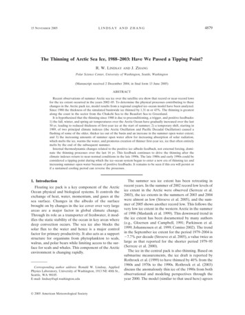
15 NOVEMBER 2005LINDSAY AND ZHANG4879The Thinning of Arctic Sea Ice, 1988–2003: Have We Passed a Tipping Point?R. W. LINDSAYANDJ. ZHANGPolar Science Center, University of Washington, Seattle, Washington(Manuscript received 2 December 2004, in final form 13 June 2005)ABSTRACTRecent observations of summer Arctic sea ice over the satellite era show that record or near-record lowsfor the ice extent occurred in the years 2002–05. To determine the physical processes contributing to thesechanges in the Arctic pack ice, model results from a regional coupled ice–ocean model have been analyzed.Since 1988 the thickness of the simulated basinwide ice thinned by 1.31 m or 43%. The thinning is greatestalong the coast in the sector from the Chukchi Sea to the Beaufort Sea to Greenland.It is hypothesized that the thinning since 1988 is due to preconditioning, a trigger, and positive feedbacks:1) the fall, winter, and spring air temperatures over the Arctic Ocean have gradually increased over the last50 yr, leading to reduced thickness of first-year ice at the start of summer; 2) a temporary shift, starting in1989, of two principal climate indexes (the Arctic Oscillation and Pacific Decadal Oscillation) caused aflushing of some of the older, thicker ice out of the basin and an increase in the summer open water extent;and 3) the increasing amounts of summer open water allow for increasing absorption of solar radiation,which melts the ice, warms the water, and promotes creation of thinner first-year ice, ice that often entirelymelts by the end of the subsequent summer.Internal thermodynamic changes related to the positive ice–albedo feedback, not external forcing, dominate the thinning processes over the last 16 yr. This feedback continues to drive the thinning after theclimate indexes return to near-normal conditions in the late 1990s. The late 1980s and early 1990s could beconsidered a tipping point during which the ice–ocean system began to enter a new era of thinning ice andincreasing summer open water because of positive feedbacks. It remains to be seen if this era will persist orif a sustained cooling period can reverse the processes.1. IntroductionFloating ice pack is a key component of the ArcticOcean physical and biological systems. It controls theexchange of heat, water, momentum, and gases at thesea surface. Changes in the albedo of the surfacebrought on by changes in the ice cover over very largeareas are a major factor in global climate change.Through its role as a transporter of freshwater, it modifies the static stability of the ocean in key areas wheredeep convection occurs. The sea ice also blocks thesolar flux to the water and hence is a major controlfactor for primary productivity. It also acts as a supportstructure for organisms from phytoplankton to seals,walrus, and polar bears while limiting access to the surface for seals and whales. This component of the Arcticenvironment is changing rapidly.Corresponding author address: Ronald W. Lindsay, AppliedPhysics Laboratory, University of Washington, 1913 NE 40th St.,Seattle, WA 98105.E-mail: lindsay@apl.washington.edu 2005 American Meteorological SocietyJCLI3587The summer sea ice extent has been retreating inrecent years. In the summer of 2002 record low levels ofice extent in the Arctic were observed (Serreze et al.2003), the ice extents in the summers of 2003 and 2004were almost as low (Stroeve et al. 2005), and the summer of 2005 shows another record low. This follows thevery low ice extent in the western Arctic in the summerof 1998 (Maslanik et al. 1999). This downward trend inthe ice extent has been documented by many authors(e.g., Gloersen and Campbell, 1991; Parkinson et al.1999; Johannessen et al. 1999; Comiso 2002). The trendin the September ice extent for the period 1979–2004 is 7.7% per decade (Stroeve et al. 2005), a value twice aslarge as that reported for the shorter period 1979–95(Serreze et al. 2000).The ice in the central pack is also thinning. Based onsubmarine measurements, the ice draft is reported byRothrock et al. (1999) to have thinned by 40% from the1960s and 1970s to the 1990s. Rothrock et al. (2003)discuss the anomalously thin ice of the 1990s from bothobservational and modeling perspectives through theyear 2000. The model (similar to that used here) agrees
4880JOURNAL OF CLIMATEVOLUME 18well with observations averaged over entire cruises andshows a thinning of the ice from 1988 to 1996. Furthermore, they compared the outputs from eight differentmodels with results published in the scientific literatureand found that they all show a local thickness maximumin 1987 and mostly thinning since then. As shown here,in recent years the ice has continued to thin at a considerable rate.The mean circulation of the ice is illustrated bymodel simulations of the mean winter and summer icevelocities, which include assimilation of ice velocitydata as described in section 2 (Fig. 1). The winter circulation is dominated by the anticyclonic Beaufort gyrein the Pacific sector of the basin (see Fig. 2 for locationnames) and the transpolar drift stream, which transports ice out of the gyre and into Fram Strait. FramStrait is the primary location for ice export from thebasin. In the summer the circulation is much weakerFIG. 2. The gray ocean region depicts the model domain. Thecross-hatched area is the Arctic Ocean, the averaging region usedfor this study.FIG. 1. Mean ice velocity for the period 1979–2003 in the winter(Oct–Apr) and summer (May–Sep). The anticyclonic Beaufortgyre is on the left and the Transpolar Drift Stream is in the centeror on the right side of the Arctic Ocean.and the Beaufort gyre is smaller and is constrainedmostly to the Beaufort Sea. The transpolar drift streamis much weaker and a small cyclonic gyre develops inthe eastern part of the basin.The drift of the ice is strongly dependent on the windspeed and direction (Thorndike and Colony 1982). Forexample, Thomas (1999) found that 56% of the variance of the ice velocity can be explained by a linearregression with the surface geostrophic wind. The geostrophic wind is determined by the surface sea levelpressure (SLP) field. To summarize the large-scale temporal changes in the Northern Hemisphere SLP,Thompson and Wallace (1998) introduced the conceptof the Arctic Oscillation (AO). The AO index is thetime series of the first principal component of theNorthern Hemisphere SLP. This component is associated with the first empirical orthogonal function (EOF)of SLP, which is an annular mode centered on the Arctic. In high AO periods the SLP is lower near the poleand the air temperature is higher in the Greenland–Iceland–Norwegian seas, the Barents Sea, and in eastern Siberia. The temperature is lower in northeasternCanada. The winter AO index changed to a stronglypositive mode in 1989 and remained positive for 7 yr.The AO is closely related to another climate index,the North Atlantic Oscillation (NAO) (Hurrell 1995),which is largely determined by the strength of the Icelandic low.The mean ice drift changes significantly with the AO(Rigor et al. 2002). When the AO index is high, the SLPBeaufort anticyclone is usually weaker and the Beaufort gyre ice circulation is usually weaker and displacedcloser to the Alaskan coast. The transpolar drift stream
15 NOVEMBER 2005LINDSAY AND ZHANGis also usually weaker; it is displaced nearer to the center of the basin and it swings more toward the northcoast of Greenland before exiting the basin throughFram Strait. Zhang et al. (2000) find a strong dependence of the ice drift and modeled thickness patternswith the NAO. In another study Zhang et al. (2004)find that in global model simulations the heat inflowfrom the south over the Iceland–Scotland Ridge (ISR)is strongly correlated with the NAO. This heat flow hascontributed to the continued thinning of Arctic sea icesince 1965. The ISR heat flow influences the ice thickness with a lag of 2–3 yr.A second climate index that is important for Arcticsea ice is the Pacific Decadal Oscillation (PDO) (Mantua et al. 1997). This index is based on the first EOF ofthe sea surface temperature in the North Pacific Ocean.The PDO is characterized by year-to-year persistenceand shows positive/warm or negative/cool values thattend to prevail for 20–30-yr periods. However, withinthese periods there are several short-lived sign reversals, including 3- or 4-yr reversals from 1958 to 1961 andagain from 1989 to 1991. The SLP in the North Pacificis correlated with the PDO and exhibits a strongerAleutian low during the positive (warm) PDO phase.Here we show (section 6b) that the sea ice thickness inthe Pacific sector of the Arctic Ocean, most notablyfrom the east Siberian Sea to the pole, is well correlatedwith the winter PDO with a lag of 1 yr.Köberle and Gerdes (2003) investigate the relativeimportance of the thermodynamic and dynamic forcings by holding either the monthly mean temperaturesor the monthly mean winds to climatological values inmodel simulations. They find that the wind-forced andthe thermally forced solutions for the total ice volumesum to give the total variation in the ice volume whenboth forcings are allowed interannual variability, indicating that the interaction of the wind-driven and thethermally driven changes is negligible. They also findthat the variability of the ice volume due to the twoforcings is similar but that specific episodes of ice thickening or thinning are created more by one or the otherof the forcings.With the same model described here (without dataassimilation) Rothrock and Zhang (2005) examined thetrend in the total hemispheric ice volume over the period 1948–99; two model simulations were performed:one with interannually varying winds and surface temperatures and one with no interannual variation of thetemperature. Using the results of Köberle and Gerdes(2003), they find that the wind-forced component of thetrend is very small and the temperature-forced component has a significant downward trend of 3% per decade.4881Holloway and Sou (2002) argue that the decreaseobserved in the submarine ice draft record by Rothrocket al. (1999) is caused by aliased sampling of the spatialand temporal variability of the ice thickness. They suggest that the timing and cruise tracks of the submarinesaliased a dominant mode of variability that consists ofan oscillation between the Canadian sector and the central and Siberian sectors of the basin. However, Rothrock et al. (2003) report good agreement in the temporal changes in ice thickness between model simulationsand the submarine observations and a basinwide thinning of the ice over the period 1987–97.Here we argue that the recent considerable retreat ofthe summer ice extent and the continual rapid declinein the mean ice thickness is not a simple responses toeither the thermodynamic forcing or the dynamic forcing, but an internal response of the system itself. Thisinternal response was manifest when the slowly changing thermodynamic forcing created consistently thinnerfirst-year ice at the start of the melt season and wastriggered by a temporary change in the ice circulationpatterns. The continual recent decline is not stronglydependent on either external forcing mode but is maintained and amplified by ice–albedo feedback processeswithin the ice–ocean system. The large changes thatbegan in 1989 suggest that the system had reached atipping point, a state of the system for which temporarychanges in the external forcing (dynamics) created alarge internal response that is no longer directly dependent on the external forcing and is not easily reversed.Of course conclusive evidence that the system did begina long-term change in the late 1980s will require manyadditional years of observations.The model and data assimilation methods are described briefly and comparisons with the observed icedraft measurements are discussed in section 2. In section 3 we introduce the model results and show how theice reduction is partitioned between level and ridged icecategories. In section 4 the processes contributing tochanges in the mean ice thickness over the 56-yr periodare presented in order to provide a longer-term contextin which to examine the recent thinning: thicknesschanges are partitioned into thermodynamic and dynamic effects, and the energy budget of the ice is examined. In section 5 an analysis of the recent considerable thinning in terms of the preconditioning, the trigger, and the response is presented. Further aspects ofthe recent thinning, including spatial characteristics, relationships to climate indexes, export at the FramStrait, and recent air temperature trends are given insection 6. Finally, comments and conclusions are givenin section 7.
4882JOURNAL OF CLIMATE2. Model description and dataWe use a coupled ice–ocean model that has beenused in a wide range of studies. The ice model is amulticategory ice thickness and enthalpy distributionmodel that consists of five main components: 1) a momentum equation that determines ice motion, 2) a viscous–plastic ice rheology with an elliptical yield curvethat determines the relationship between ice deformation and internal stress, 3) a heat equation that determines ice temperature profile and ice growth or decay,4) two ice thickness distribution equations for deformed and undeformed ice that conserve ice mass, and5) an enthalpy distribution equation that conserves icethermal energy. The first two components are described in detail by Hibler (1979). The ice momentumequation was solved using Zhang and Hibler’s (1997)numerical model for ice dynamics. The heat equationwas solved, over each category, using Winton’s (2000)three-layer thermodynamic model, which divides theice in each category into two layers of equal thicknessbeneath a layer of snow. The ice thickness distributionequations are described in detail by Flato and Hibler(1995). The ocean model is based on the Bryan–Coxmodel (Bryan 1969; Cox 1984) with an embeddedmixed layer of Kraus and Turner (1967). Detailed information about the ocean model is found in Zhang etal. (1998) and about the enthalpy distribution model isin Zhang and Rothrock (2001).The model domain (Fig. 2) covers the Arctic Ocean,the Barents and Kara Seas, and the Greenland–Iceland–Norwegian seas. It has a horizontal resolutionof 40 km 40 km, 21 ocean levels, and 12 thicknesscategories each for undeformed ice, ridged ice, ice enthalpy, and snow. The ice thickness categories, themodel domain, and bottom topography can be found inZhang et al. (2000). The model is forced with dailyfields of sea level air pressure (SLP) and 2-m air temperature (T2m) obtained from the National Centers forEnvironmental Prediction–National Center for Atmospheric Research (NCEP–NCAR) reanalysis (Kalnayet al. 1996) for the 56-yr period 1948–2003. The seasonally varying drag coefficient follows that of Overlandand Colony (1994) with a minimum value of 0.97 10 3 in the winter and a maximum of 1.42 10 3 in thesummer. The specific humidity and longwave andshortwave radiative fluxes are calculated following themethod of Parkinson and Washington (1979) based onthe SLP and T2m fields. The cloud fractions used tocompute the downwelling radiative fluxes only haveseasonal variability and no spatial or interannual variability. Model input also includes river runoff and pre-VOLUME 18cipitation detailed in Hibler and Bryan (1987) andZhang et al. (1998).The ice concentration is assimilated from an ice concentration dataset originally created by Chapman andWalsh (1993). The dataset, the Global Sea Ice (GICE)dataset [a more recent version is the Hadley Centre SeaIce and Sea Surface Temperature (HadISST) dataset;Rayner et al. (1996)], is obtained from the British Atmospheric Data Center. It consists of monthly averagedice concentration on a 1 grid. In the satellite era (1979–2003) it is based largely on visible, infrared, and passivemicrowave measurements, and in the presatellite era onship reports and climatology. For 2003 only we use theHadISST ice concentrations because the GICE datasetends in 2002. We use data from 1948 to 2003 and linearly interpolate the monthly data to daily intervals.This interpolation method smoothes extreme values ofthe concentration, reduces the variability, and does notalways maintain the reported monthly mean value(Taylor et al. 2000).The assimilation procedure is outlined in Lindsayand Zhang (2005). Each day the model estimate Cmod isnudged to a revised estimate Ĉmod with the relationshipĈmod Cmod K共Cobs Cmod兲,共1兲and the gain (or weighting) function isK ⱍCobs Cmodⱍ ⱍCobs Cmodⱍ R2,共2兲where Cobs is the observed concentration, R2 is the error variance of the observations, and the exponent 6. This large exponent means that, only if the differencebetween the observations and the model is greater thanabout 0.5, are the observations heavily weighted, in effect only assimilating the ice extent. We use a fixedvalue of R 0.05 that is consistent with the estimatederrors of the GICE dataset. Changes in the thicknessdistribution were made to accommodate the change inthe ice concentration in a manner that minimizedchanges in the ice mass by removing or adding ice to thethinnest ice classes.Ice velocity measurements are assimilated with anoptimal interpolation scheme outlined in Zhang et al.(2003). We use velocity measurements from both buoyderived and Special Sensor Microwave Imager (SSM/I)-derived ice displacement data. The buoy velocitieswere obtained from the International Arctic Buoy Program (IABP), and SSM/I 85-GHz ice displacementmeasurements were provided by the Jet PropulsionLaboratory Polar Remote Sensing Group. The buoyvelocities are 24-h averages and the SSM/I velocitiesare based on 2-day displacements. The passive microwave displacement estimates are based on a maximum
15 NOVEMBER 2005LINDSAY AND ZHANGcorrelation method applied to sequential images of theice cover. While the SSM/I daily velocity estimates havea substantially larger error standard deviation than thebuoys (0.057 versus 0.007 m s 1), their large numberand excellent spatial coverage make them a valuableaddition to our analysis.Lindsay and Zhang (2005, manuscript submitted to J.Atmos. Oceanic Technol., hereafter LIN05) alsopresent comparisons between modeled and submarinemeasurements of ice draft; simulations were modelonly or included assimilation of ice concentration(1948–2003) or assimilation of both ice concentrationand velocity (1979–2003). The comparisons of themodel and the observed ice draft are progressively improved with the assimilation of each variable. In theperiod 1987–97 the model-only simulation of the icedraft has a bias of 0.11 m and a correlation of R 0.51 (N 835 50-km segments). With assimilation ofice concentration the bias is 0.30 m and the correlation is R 0.63. When ice velocity is also assimilated,the bias is reduced to 0.02 m and the correlation increases to 0.70; the rms difference is 0.76 m. There is astrong spatial pattern in the bias of the model ice draftcompared to the submarine ice draft, with the modelshowing ice too thick on the Pacific side of the basinand too thin on the Atlantic side. The spatial pattern ofthe model bias is puzzling because it persists even whenice velocity measurements are assimilated and hencethe mean advective patterns are well estimated. Thissuggests that there may be some large-scale error in themodel forcing or in the model physics.Here we use the assimilation of ice concentrationduring the whole period of study and assimilation of icevelocity beginning in 1979 when ice velocity observations became abundant. Note that the assimilation ofice concentration and velocity did not greatly changethe mean ice thickness simulations. The prominentmaxima in 1966 and 1987 and the rapid decline in icethickness since 1987 are present in all three simulations.The assimilation of ice velocity beginning in 1979 introduces an increase in the mean ice thickness of about0.3 m over that of the assimilation of ice concentrationalone; however our primary period of interest is 1988–2003, well after this change in the assimilation procedures. We use assimilation of both ice concentrationand velocity to obtain a better representation of thedetails of the changes in the ice in this 16-yr period.3. Model results: Changes in the mean thicknessIn the model simulations one-third to one-half of theice volume in the Arctic Basin is ridged ice and the restis level ice. Figure 3 shows the time series of the meanice thickness in the Arctic Ocean and the mean thick-4883FIG. 3. Annual mean ice thickness (over the total area of theArctic Ocean) of all ice, level ice, and ridged ice. The vertical linesindicate the times of the two principal maxima and are used insubsequent figures for reference.ness (over the entire area) of level and ridged ice. Since1988 the basinwide thickness has thinned by 1.31 m.During this period the volume of ridged ice has diminished more rapidly than that of the level ice. The levelice has been on a downward trend since 1966, but theridged ice volume peaked in 1987 and 1988 and hasfallen sharply since. The volume fraction of the ridgedice has fallen from 54% in 1988 to 46% in 2003. Thisresult is consistent with the modeling studies of Makshtas et al. (2003) who also report that most of thedecrease in sea ice thickness is caused by a decrease inridged ice and an increase in the area of undeformedice. Rothrock and Zhang (2005) report that a decline inthe ice volume of level ice predominates. Rigor andWallace (2004) explain the low summer sea ice extentsof recent years as a delayed response to the high-indexAO years of 1989–95 and to a change of the average ageof the ice in the basin, a change that would also implya decrease in the ridged ice volume.The ice has thinned over almost all of the basin. Atthe time of the annual mean thickness maximum in1987 and 1988 the mean ice thickness is at least 2.5 mover the entire central part of the basin, while in 2003very little ice is greater than 2 m thick (Fig. 4). A narrow band of thick ice remains along the Canadian coast.FIG. 4. Annual mean ice thickness for 1988 and 2003.
4884JOURNAL OF CLIMATEFIG. 5. Trend in the ice thickness for the 16-yr period1988–2003 for all ice, level ice, and ridged ice.Looking at just these 2 yr, the ice has thinned most inthe east Siberian Sea, but the trend is quite differentbecause it is derived from a linear fit of the ice thicknesswith time. For the 16 yr after 1988 the greatest trendsare in the Beaufort Sea and along the Canadian coast(Fig. 5). There is a large reduction in the ridged-icevolume all along the Alaskan, Canadian, and Greenland coasts while the level-ice volume was reduced onlyslightly in the same period. The trend in the mean thickness is almost all due to the trend in ridged ice. Significance tests for the trend are not appropriate becausethe time interval analyzed is subjectively chosen to startwith a maximum in the mean ice thickness and to specifically include a time when the trend is large. Clearlythe trend in the basinwide mean thickness is greater inthis 16-yr period than in any other 16-yr period in the56-yr simulation (Fig. 3). Irrespective of the statisticalsignificance of this trend, we are interested in the physical processes contributing to it.The thinning trend for the 16 yr since 1988 is muchVOLUME 18different from the trend for the full 56-yr simulationpresented in LIN05 or Rothrock and Zhang (2005),which both show the thinning rate was greatest in thearea north of the east Siberian and Laptev Seas andextended in a broad band to Fram Strait. Here, themore recent 16-yr period shows that the ice in the Siberian sector is generally thin first-year ice and the thinning trends are smaller in this sector than in the Canadian sector where ridged ice prevails. The maximumthinning rates are about 0.04 m yr 1 for the 56-yrperiod, while in the latest 16-yr period the maximumrates are 3 times as high, about 0.12 m yr 1.The model has 12 ice thickness bins that determinethe ice thickness distribution. Comparisons of the thickness distributions for the whole Arctic Ocean for 1987and 2003 show considerable changes. The mode is thebin with the largest area fraction. In May, at the start ofthe melt season, the mode is reduced by half, from 1.5to 0.7 m. The ice is more concentrated in the thin bins:22% more of the area is covered by ice less than 2 mthick. These simulations are supported by observations.Yu et al. (2004) report that observations of ice draftfrom submarines over the periods 1958–70 (a period ofrelatively thick ice) and 1993–97 (a period of rapidlythinning ice) also show a substantial loss of ice thickerthan 2 m and increases in the amount of ice in the1–2-m range. As reported here, they find the area fraction loss is greatest for the thickest ice categories.Bitz and Roe (2004) argue that any change in theexternal forcing that thins the ice independent of itsthickness causes the annual mean thickness of the thickice to diminish more than that of the thin ice because ofthermodynamic effects. For example, if the net energyflux to the ice increases, the anomalous increase in meltof thick and thin ice are comparable (as long as the thinice does not melt away entirely), but thin ice respondsby growing anomalously much faster in the winter.Hence, we would expect thicker ridged ice to diminishfaster than thinner level ice under an increase in the netenergy flux or, as explained by Bitz and Roe (2004), ifice divergence increases uniformly for all ice thicknesses.4. Processes contributing to ice thickness changea. Advection and thermodynamic growthChanges in the mean ice thickness at each grid cellcan be partitioned into two components: one due to thenet advection and one due to thermodynamics. The netadvection, or mass-flux convergence, is hadv 冕t tt · hu dt,共3兲
15 NOVEMBER 2005LINDSAY AND ZHANGFIG. 6. Mean annual thickness changes due to thermodynamicgrowth or melt and net advection per year for winter (Oct–Apr)and summer (May–Sep) for the 56-yr period 1948–2003.where u is the vector velocity, h is the mean ice thickness, and t is the time interval. The thermodynamicgrowth or melt is htdg 冕t t nbinst兺 关 g共h 兲f共h 兲 共h 兲兴 dt,iii共4兲i 1where the summation is over the thickness bins andg(h) is the thickness distribution, f(h) is the thermodynamic growth rate, and (h) is the lateral melt rate. Thenet thickness change over the interval is then h hadv htdg.共5兲These terms of the ice mass balance have significantspatial and seasonal variability, as might be expected.Figure 6 shows the mean annual change in the thicknessdue to each of the two terms for the winter and summerseasons from the 56-yr simulation. There is net growthof 1 m or more over much of the basin in the winter anda lesser amount of melt in the summer. The net advection is quite small but slightly negative over most of thecentral part of the basin due to a small net divergence,divergence accommodated by the export of ice throughFram Strait. The region of greatest winter growth is inthe Laptev Sea and in portions of the Kara and BarentsSeas where more than 3 m of ice grows each winter.These are locations where there is often significant offshore flow and the continual creation of shore polynyas. Because of the winter offshore flow, the westernLaptev is also a region of net advective loss in the winter but not in the summer when the winds are morevariable. The eastern edge of the East Greenland Cur-4885rent exhibits strong advective gain in both winter andsummer, as well as strong melt in both seasons. Another region of strong advective gain in the winter is inthe Chukchi Sea, where the anticyclonic Beaufort gyrebrings thicker ice into the shelf region. Similarly, anadvective loss is seen in the eastern Beaufort Sea wherethe gyre is pulling thick ice away from the coast.These terms also show significant interannual variability. The annual total thermodynamic growth andnet export, averaged over the Arctic Ocean (Figs. 7aand 7b), show the average winter growth is 1.30 m yr 1and the average summer melt is 0.91 m yr 1. The netadvection is nearly zero in the summer and negative inthe winter, averaging 0.41 m yr 1. This term represents the net export of ice from the basin. The averagethinning rate due to both processes over the entire 56yr period is 0.02 m yr 1.The net change in the ice thickness is determined bythe difference in the cumulative effect of large terms.Over the 56 yr of simulation, the thermodynamic wintergrowth totals 73 m of ice. This is balanced by summermelt and net advection to produce a net change of just 0.79 m (Fig. 3). So how, when, and where is the netchange produced? To determine the integrative effectof anomalous periods of thickness change contributedby each of these terms we compute the cumulativeanomaly from the mean (Figs. 7c and 7d). This type ofplot simply shows periods of abnormal growth or meltwhen one of the terms is contributing more or less thannormal to the change of the ice thickness. When the lineis sloping upward (positive anomalies), the term is contributing to thickening of the ice more than average(either through more growth, less melt, or less advective loss than average) and, when the line is slopingdown, it is contributing to thinning of the ice more thanaverage (either through less growth, more melt, ormore advective loss than average). By definition theseplots must begin and end at zero. A consistent upwardtrend in one of the terms will appear as first a downward-sloping line (the anomalies are negative) and thenan upward-sloping line (the anomalies are positive).The sum of the annual lines in the cumulative plotsreproduces the shape of the mean ice thickness line inFig. 3 without the long-term 56-yr trend. The summermelt anomalies represent the largest contribution to thecumulative interannual variability of the thicknesschanges. There is a
considered a tipping point during which the ice-ocean system began to enter a new era of thinning ice and increasing summer open water because of positive feedbacks. It remains to be seen if this era will persist or if a sustained cooling period can reverse the processes. 1. Introduction Floating ice pack is a key component of the Arctic