Transcription
Using Python in Climateand MeteorologyJohnny Wei-Bing LinPhysics Department, North Park Universitywww.johnny-lin.comAcknowledgments: Many of the CDAT-related slides are copied or adaptedfrom a set by Dean Williams and Charles Doutriaux (LLNL PCMDI). Thanksalso to the online CDAT documentation, Peter Caldwell (LLNL), and AlexDeCaria (Millersville Univ.).Slides version date: June 20, 2011. Author email: johnny@johnny-lin.com. Presentedat National Taiwan University, Taipei, Taiwan. This work is licensed under a CreativeCommons Attribution-NonCommercial-ShareAlike 3.0 United States License.
Outline Why Python?Python tools for data analysis: CDAT.Using Python to make models moremodular: The qtcm example.
Why Python?: Topics What is Python?Advantages and disadvantages.Why Python is now gaining momentum inthe atmospheric-oceanic sciences (AOS)community.Examples of how Python is used as ananalysis, visualization, and workflowmanagement tool.
What is Python? Structure: Is a scripting, procedural, as wellas a fully native object-oriented (O-O)language.Interpreted: Loosely/dynamically-typed andinteractive.Data structures: Robust built-in set and usersare free to define additional structures.Array syntax: Similar to Matlab, IDL, andFortran 90 (no loops!).Platform independent, open-source, and free!
Python's advantages Concise but natural syntax, both arrays and non-arrays,makes programs clearer. “Python is executablepseudocode. Perl is executable line noise.”Interpreted language makes development easier.Object-orientation makes code more robust/less brittle.Built-in set of data structures are very powerful and useful(e.g., dictionaries).Namespace management which prevents variable andfunction collisions.Tight interconnects with compiled languages (Fortran viaf2py and C via SWIG), so you can interact with compiledcode when speed is vital.Large user and developer base in industry as well asscience (e.g., Google, LLNL PCMDI).
Python's disadvantages Runs much slower than compiled code (but there are toolsto overcome this).Relatively sparse collection of scientific libraries comparedto Fortran (but this is growing).
Why AOS Python is now gaining momentum Python as a language was developed in the late 1980s, but even as lateas 2004, could be considered relatively “esoteric.”But by 2005, Python made a quantum jump in popularity, and hascontinued to grow.Now is ranked 8th in the June 2011 TIOBE Programming CommunityIndex (which indicates the “popularity” of languages). Fortran is ranked33rd, Matlab 23rd, and IDL is in the undifferentiated 50-100th group.http://www.paulgraham.com/pypar.html, on.html
Why AOS Python is now gaining momentum (cont.) Around the same time, key tools for AOS use becameavailable: In 2005, NumPy was developed which (finally) provided astandard array package.SciPy was begun in 2001 and incorporated NumPy to createa one-stop shop for scientific computing.CDAT 3.3 was released in 2002, which proved to be theversion that really took off (the current version is 5.2).PyNGL and PyNIO were developed in 2004 and 2005,respectively.matplotlib added a contouring package in the mid-2000's.http://www.scipy.org/History of SciPyhttp://www.pyngl.ucar.edu/Images/history.png
Why AOS Python is now gaining momentum (cont.) Institutional support in the AOS community now includes: Lawrence Livermore National Laboratory's Program forClimate Model Diagnosis and Intercomparison (LLNLPCMDI) produces CDAT, etc.National Center for Atmospheric Research Computationaland Information Systems Laboratory (NCAR CISL) producesPyNGL and PyNIO.Center for Ocean-Land-Atmosphere Studies/Institute ofGlobal Environment and Society (COLA/IGES) producesPyGrADS.American Meteorological Society (AMS): Sponsored anAdvances in Using Python symposium at the 2011 AMSAnnual Meeting (the symposia will reprise in 2012) as well asa Python short course.AOS Python users can now be found practically anywhere.An overview of AOS Python resources is found at thePyAOS website: http://pyaos.johnny-lin.com.
Example of visualization: Skew-T andmeteograms All plots on this slide are produced by PyNGL and taken from their web site.See http://www.pyngl.ucar.edu/Examples/gallery.shtml for code.
Example of visualization and delivery of weathermaps of NWP model results Screenshots taken from the WxMAP2 package web site.http://sourceforge.net/projects/wxmap2/
Example of analysis and visualization:Provenance managementSession of the VisTrails visualization and data workflow andprovenance management system; salinity data in the Columbia Riverestuary is graphed.http://www.vistrails.org/index.php?title File:Corie example.png&oldid 616
Example of analysis, visualization, and workflowmanagement and integration Problem: Many different components of the Applied Climate InformationSystem: Data ingest, distribution, storage, analysis, web services.Solution: Do it all in Python: A single environment of shared state vs. acrazy mix of shell scripts, compiled code, Matlab/IDL scripts, and webserver makes for a more powerful, flexible, and maintainable system.Image from: AMS talk by Bill Noon, Northwest Regional Climate Center, Ithaca, gi/id/17853?recordingid 17853
Outline Why Python?Python tools for data analysis: CDAT.Using Python to make models moremodular: The qtcm example.
Python tools for data analysis: TopicsWe will look at only one tool (the Climate Data AnalysisTools or CDAT) and a few aspects of how that tool helpsus with data analysis: What is CDAT? Dealing with missing data: Masked arrays andvariables. Comparing different datasets: Time axis alignment. Dealing with different grids: Vertical interpolation,regridding. What is VCDAT? A walk through simple analysis using VCDAT.
What is CDAT? Written by LLNL PCMDI and designed for climate sciencedata, CDAT was first released in 1997.Unified environment based on the object-oriented Pythoncomputer language.Integrated with packages that are useful to theatmospheric sciences community: Climate Data Management System (cdms).NumPy, masked array (ma), masked variable (MV2)Visualization (vcs, Xmgrace, matplotlib, VTK, Visus, etc.And more! (i.e., OPeNDAP, ESG, etc.).Graphical user interface (VCDAT).XML representation (CDML/NcML) for data sets.Community software (BSD open source license).URL: http://www-pcmdi.llnl.gov/software-portal.
Dealing with missing data: Why maskedarrays and masked variables? Python supports array variables (via NumPy).All variables in Python are not technically variables,but objects: Objects hold multiple pieces of data as well as functions thatoperate on that data.For AOS applications, this means data and metadata (e.g.,grid type, missing values, etc.) can both be attached to the“variable.”Using this capability, we can define not only arrays,but two more array-like variables: masked arrays andmasked variables.Metadata attached to the arrays can be used as partof analysis, visualization, etc.
What are masked arrays and maskedvariables?
How do masked arrays and maskedvariables look and act in Python? import numpy as N a N.array([[1,2,3],[4,5,6]]) aarray([[1, 2, 3],[4, 5, 6]])Arrays: Every elementhas a value, andoperations using thearray are definedaccordingly. import numpy.ma as ma b ma.masked greater(a, 4) bmasked array(data [[1 2 3][4 ]],mask [[False False False][False True True]],fill value 999999) print a*b[[1 4 9][16 ]]Masked arrays: A maskof bad values travelswith the array. Thoseelements deemed badare treated as if they didnot exist. Operationsusing the arrayautomatically utilize themask of bad values.
How do masked arrays and maskedvariables look in Python (cont.)?Additionalinfo such as:MetadataAxes import MV2 d MV2.masked greater(c,4) d.info()*** Description of Slab variable 3 ***id: variable 3shape: (3, 2)filename:missing value: 1e 20comments:grid name: N/Agrid type: N/Atime statistic:long name:units:No grid present.** Dimension 1 **id: axis 0Length: 3First: 0.0Last:2.0Python id: 0x2729450[. rest of output deleted for space .]
Comparing different datasets: Time axisalignment Different datasets and model runs can have ways of specifyingtime, e.g., different: CDAT time axis values can be referenced in two ways: Relative time: A number relative to a datum (e.g., 10 months sinceJan 1, 1970).Component time: A date on a specific calendar (e.g., 1970-10-01).If t is your time axis (via getTime): Calendars: Gregorian, Julian, 360 days/year, etc.Starting points: Since 1 B.C./A.D. 1, since Jan 1, 1970, etc.To change to the same relative time datum, e.g.:t.toRelativeTime('months since 1800 01 01')To change to component time based on a specified calendar, e.g.:t.asComponentTime(calendar cdtime.DefaultCalendar)From there, you can subset either on the basis of the samerelative time values or for a given component time date.
Dealing with different grids Vertical interpolation:P , B, P0)P cdutil.vertical.linearInterpolation(var, depth,levels)P cdutil.vertical.logLinearInterpolation(var,depth, levels) Vertical regridding: Use the MV2 pressureRegrid method:var on new levels var.pressureRegrid(levout) Horizontal regridding: Create a grid, then use the MV2regridding method to create a variable on the new grid.E.g., from a rectangular grid to a 96x192 rectangularGaussian grid:var f(’temp’)n48 grid cdms2.createGaussianGrid(96)var48 var.regrid(n48 grid)
What is VCDAT?VariableselectionVCDAT lets you getfamiliar with manyparts of CDAT withoutlearning Python.The executable isnamed vcdat and isfound in/opt/cdat/bin.Dimensionselection andmanipulationVariable andgraphicsselection andmanipulationDean Williams and Charles Doutriaux (LLNL PCMDI)
A walk through simple analysis usingVCDAT Reading in data (local and remote)Selecting a variableSelecting axis rangesPlotting a longitude-latitude slicePlotting a time-longitude slicePlotting time vs. a regional averageBasic calculations using data (definedvariables)Saving a plotAs a tool for teaching CDAT and Python
Outline Why Python?Python tools for data analysis: CDAT.Using Python to make models moremodular: The qtcm example.
Traditional AOS model coding techniquesand tools Written in compiled languages (often Fortran): Pros: Fast, "standard," free, many well-tested libraries.Cons: Natively procedural, limited data structures (relateddata are not related to each other), non-interactive, portabilityissues (F90 standard does not specify memory allocation fornon-standard data structures and each compiler implementsdifferent features differently).Language choice affects development cycle.Interfacing with operating system often unwieldy,through shell scripts, makefiles, etc.Substantial amounts of very old legacy code.Parallelization requires the climate scientist to dealwith processor and memory management (MPI)issues.
Traditional practices yield problematic andunmodular code Brittle: Errors and collisions are common.Difficult for other users (even yourself a fewmonths/years later!) to understand.Difficult to extend: Interfaces are poorly defined andstructured between: Submodels (e.g., between atmosphere and ocean)Subroutines/procedures in a modelModels and the operating systemModels and the user (in terms of the user's thinkingprocesses)Non-portable: Difficult for models and sub-models totalk to one another, sometimes even on the sameplatform.
Capabilities of Python to help modularizemodels Object-orientation: Makes it easier to develop robust and multiapplication interfaces between tools, and, in theory, more closelyapproximate human mental representations of the world.Interpreted and dynamically-typed: Enables run time alterationof variables, as well as the reuse of code in multiple contexts(e.g., c a*b works properly in a routine without changeregardless of what type, size, and rank a and b are).Shared state: You can access virtually all variables. Note this isnot some sort of giant common block, because namespacemanagement and object decomposition automatically protectfrom collisions and accidental overwriting.Built-in set/collection data structures (i.e., lists, dictionaries)greatly improve the flexibility of the code.Clarity of syntax: Code is more robust and modules developedfor different applications can be more easily reused.
Example of modularizing a model withPython: The qtcm atmospheric model Originally there was QTCM1, the Neelin-Zeng QuasiEquilibrium Tropical Circulation Model (Neelin & Zeng1999 and Zeng et al. 1999).Intermediate-level atmospheric modelWritten in Fortran.Vertical temperature and moisture profiles basedupon convective quasi-equilibrium assumption.Resolution 5.625 deg longitude, 3.75 deg latitude.Includes a simple radiative code and a Betts-Miller(1986) type convective scheme.Reasonable simulation of tropical climatology and alsoincludes Madden-Julian oscillation (MJO)-likevariability.
The qtcm atmospheric model (cont.) qtcm is a Python wrapping of QTCM1: Connectivity: Through the program f2py: Fortran: Numerics of QTCM1.Python: User-interface wrapper that managesvariables, routine execution order, runs, and modelinstances.Almost automatically makes the Fortran routines andmemory space available to Python.You can set Fortran variables at the Python level, evenat run 2-12009.html
qtcm features: A simple qtcm runfrom qtcm import Qtcminputs {}inputs['runname'] 'test'inputs['landon'] 0inputs['year0'] 1inputs['month0'] 11inputs['day0'] 1inputs['lastday'] 30inputs['mrestart'] 0inputs['compiled form'] 'parts'model Qtcm(**inputs)model.run session()Configuration keywords in thisrun yield: The output filenames willcontain the string given byrunname. Aquaplanet (set by landon). Start from Nov 1, Year 1.Run for 30 days. Start from a newly initializedmodel state.Run the model using therun session method.compiled form keywordchooses the model version thatgives control down to theatmospheric timestep.
qtcm features: Run sessions and acontinuation run in qtcminputs['year0'] 1inputs['month0'] 11inputs['day0'] 1inputs['lastday'] 10inputs['mrestart'] 0inputs['compiled form'] 'parts'model Qtcm(**inputs)model.run session()model.u1.value model.u1.value * 2.0model.init with instance state Truemodel.run session(cont 30) One run session is conducted with the model instance.The value of u1, the baroclinic zonal wind, is doubled.A continuation run is made for 30 more days.All this can be controlled at runtime, and interactively.
qtcm features: Multiple qtcm model runsusing a snapshot from a previous runsessionmodel.run session()mysnapshot model.snapshotmodel1.sync set py values to snapshot(snapshot mysnapshot)model2.sync set py values to snapshot(snapshot mysnapshot)model1.run session()model2.run session() Snapshots are variables (dictionary objects) that act asrestart files.model1 and model2 are separate instances of theQtcm class and are truly independent (they share novariables or memory).Again, objects enable us to control model configurationand execution in a clear but powerful way.
qtcm features: Runlists make the modelvery modular model Qtcm(compiled form ’parts’) print model.runlists[’qtcminit’][' qtcm.wrapcall.wparinit’,’ qtcm.wrapcall.wbndinit’, ’varinit’,{’ qtcm.wrapcall.wtimemanager’: [1]}, ’atm physics1’] Runlists specify a series of Python or Fortran methods,functions, subroutines (or other run lists) that will be executedwhen the list is passed into a call of the run list method.Routines in run lists are identified by strings (instead of, forinstance, as a memory pointer to a library archive object file) andso what routines the model executes are fully changeable atrun time.The example shows a list with two Fortran subroutines withoutinput parameters, a Python method without input parameters, aFortran subroutine with an input parameter, and another run list.
qtcm benefits: Improving the modeling andanalysis cycle for climate modeling studies The object decomposition provides a high level of flexibilityfor changing i/o, data, variables, subroutine execution order,and the routines themselves at run time.The performance penalty of this hybrid-languge model vs.the Fortran-only version of the model is 4–9%.But for this cost, modeling is now no longer a static exercise(i.e., set parameters, run, analyze output).With modeling more dynamic, the modeling study can adaptand change as the model runs.This means that we can unify not only the traditionallycomputer-controlled portions of a modeling workflow, butalso parts of the traditionally human-controlled portions(hypothesis generation).
qtcm benefits: Improving the modeling andanalysis cycle for climate modeling studies (cont.)Traditional analysis sequence used in modeling studies:Transformed analysis sequence using qtcm-like tools:Outlined arrows mainly human input. Gray-filled arrows a mix of human andcomputer-controlled input. Completely filled (black)-arrows purely computercontrolled input.Model output analysis can now automatically control future model runs. Trydoing that with a kludge of shell scripts, pre-processors, Matlab scripts, etc.!
qtcm benefits: Modeling can be interactive Because Python is interpreted, this permits model alteration at run timeand thus interactive modeling. All variables can be changed at runtime and in the model run.Visualization can also be done interactively.
Conclusions Python is a mature, comprehensivecomputational environment for all aspectsof the atmospheric and oceanic sciences.AOS Python tools make data analysismuch easier to do.Python offers tools to make models moreflexible and capable of exploring previouslydifficult to access scientific problems.And it's (mostly) all free!
Python's advantages Concise but natural syntax, both arrays and non-arrays, makes programs clearer. “Python is executable pseudocode. Perl is executable line noise.” Interpreted language makes development easier. Object-orientation makes code more robust/less brittle. Built-in set of data stru