WIXLIB

Statistics and risk modelling using PythonEric Marsden eric.marsden@risk-engineering.org Statistics is the science of learning from experience,particularly experience that arrives a little bit at atime.— B. Efron, Stanford

Learning objectivesUsing Python/SciPy tools:1Analyze data using descriptive statistics and graphical tools2Fit a probability distribution to data (estimate distribution parameters)3Express various risk measures as statistical tests4Determine quantile measures of various risk metrics5Build flexible models to allow estimation of quantities of interest andassociated uncertainty measures6Select appropriate distributions of random variables/vectors for stochasticphenomena

Where does this fit into risk engineering?datacurvefittingprobabilistic modelconsequence modelevent probabilitiesevent consequencesrisks

Where does this fit into risk engineering?datacurvefittingprobabilistic modelconsequence modelevent probabilitiesevent consequencescostsriskscriteriadecision-making

Where does this fit into risk engineering?datacurvefittingprobabilistic modelconsequence modelevent probabilitiesevent consequencesThese slidescostsriskscriteriadecision-making

Angle of attack: computational approach to statistics Emphasize practical results rather than formulæ and proofs Include new statistical tools which have become practical thanks topower of modern computers “resampling” methods, “Monte Carlo” methods Our target: “Analyze risk-related data using computers” If talking to a recruiter, use the term data science very sought-after skill in 2019!

A sought-after skillSource: indeed.com/jobtrends

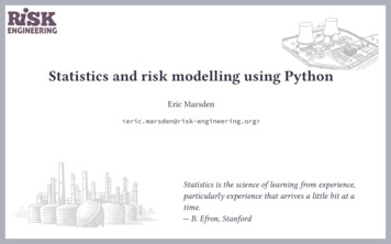
A long historyJohn Graunt collected and published publichealth data in the uk in the Bills of Mortality(circa 1630), and his statistical analysis identifiedthe plague as a significant source of prematuredeaths.Image source: British Library, public domain

Python and SciPyEnvironment used in this coursework: Python programming language SciPy NumPy matplotlib libraries Alternative to Matlab, Scilab, Octave, R Free software A real programming language with simple syntax much, much more powerful than a spreadsheet! Rich scientific computing libraries statistical measures visual presentation of data optimization, interpolation and curve fitting stochastic simulation machine learning, image processing

How do I run it? Cloud without local installation Google Colaboratory, at colab.research.google.com CoCalc, at cocalc.com Microsoft Windows: install one of Anaconda from anaconda.com/download/Python 2 or Python 3? pythonxy from python-xy.github.ioPython version 2 reached end-oflife in January 2020. You shouldonly use Python 3 now.MacOS: install one of Anaconda from anaconda.com/download/ Pyzo, from pyzo.org Linux: install packages python, numpy, matplotlib, scipy your distribution’s packages are probably fine

Google Colaboratory colab.research.google.com Runs in the cloud, access via web browser No local installation needed Can save to your Google Drive Notebooks are live computationaldocuments, great for “experimenting”

CoCalc Runs in the cloud, access via web browser No local installation needed Access to Python in a Jupyter notebook,Sage, R Create an account for free Similar tools: Microsoft Azure Notebooks JupyterHub, at jupyter.org/try cocalc.com

Python as a statistical calculatorIn [1]: import numpyIn [2]: 2 2Out[2]: 4In [3]: numpy.sqrt(2 2)Out[3]: 2.0In [4]: numpy.piOut[4]: 3.141592653589793In [5]: numpy.sin(numpy.pi)Out[5]: 1.2246467991473532e-16In [6]: numpy.random.uniform(20, 30)Out[6]: 28.890905809912784In [7]: numpy.random.uniform(20, 30)Out[7]: 20.58728078429875as aDownload this contentPython notebook atrgrisk-engineering.o

Python as a statistical calculatorIn [3]: obs numpy.random.uniform(20, 30, 10)In [4]: obsOut[4]:array([ 25.64917726,25.43993038,26.05497056,21.35270677, 21.71122725,22.72479854, 2.70541355, 43.42245451,45.44959708, 44.7032953 ,44.03009478])55.8887125 ,40.46457257,In [5]: len(obs)Out[5]: 10In [6]: obs obsOut[6]:array([ 51.29835453,50.87986076,52.10994112,In [7]: obs - 25Out[7]:array([ 0.64917726, -3.64729323, -3.28877275,0.43993038,-2.27520146, -2.64835235, -4.76771371,-2.98495261])In [8]: obs.mean()Out[8]: 23.547614834213316In [9]: obs.sum()Out[9]: 235.47614834213317In [10]: obs.min()Out[10]: 20.2322862858454832.94435625,1.05497056,

Python as a statistical calculator: plottingIn [2]: importnumpy, matplotlib.pyplot as pltIn [3]: x numpy.linspace(0, 10, 100)In [4]: obs numpy.sin(x) numpy.random.uniform(-0.1, 0.1, 100)In [5]: plt.plot(x, obs)Out[5]: [ matplotlib.lines.Line2D at 0x7f47ecc96da0 ]In [7]: plt.plot(x, obs)Out[7]: [ matplotlib.lines.Line2D at 0x7f47ed42f0f0 ]

Some basic notions inprobability and statistics

Discrete vs continuous variablesDiscreteContinuousA discrete variable takes separate, countablevaluesA continuous variable is the result of ameasurement (a floating point number)Examples:Examples: outcomes of a coin toss: {head, tail} height of a person number of students in the class flow rate in a pipeline questionnaire responses {very unsatisfied,unsatisfied, satisfied, very satisfied} volume of oil in a drum time taken to cycle from home touniversity

Random variablesA random variable is a set of possible values from a stochastic experimentExamples: sum of the values on two dice throws (a discrete random variable) height of the water in a river at time 𝑡 (a continuous random variable) time until the failure of an electronic component number of cars on a bridge at time 𝑡 number of new influenza cases at a hospital in a given month number of defective items in a batch produced by a factory

Probability Mass Functions For all values 𝑥 that a discrete random variable 𝑋 may take, wedefine the function𝑝𝑋 (𝑥) Pr(𝑋 takes the value 𝑥) This is called the probability mass function (pmf) of 𝑋Example: 𝑋 “number of heads when tossing a coin twice” 𝑝𝑋 (0) Pr(𝑋 0) 1/4 𝑝𝑋 (1) Pr(𝑋 1) 2/40.70.60.50.40.30.2 𝑝𝑋 (2) Pr(𝑋 2) 1/40.10.0012

Probability Mass Functions: two coins Task: simulate “expected number of heads when tossing a coin twice” Let’s simulate a coin toss by random choice between 0 and 1 numpy.random.randint(0, 2)1inclusive lower boundexclusive upper boundas aDownload this contentPython notebook atrgrisk-engineering.o

Probability Mass Functions: two coins Task: simulate “expected number of heads when tossing a coin twice” Let’s simulate a coin toss by random choice between 0 and 1 numpy.random.randint(0, 2)1inclusive lower bound exclusive upper boundToss a coin twice: numpy.random.randint(0, 2, 2)array([0, 1])countas aDownload this contentPython notebook atrgrisk-engineering.o

Probability Mass Functions: two coins Task: simulate “expected number of heads when tossing a coin twice” Let’s simulate a coin toss by random choice between 0 and 1 numpy.random.randint(0, 2)1inclusive lower bound exclusive upper boundToss a coin twice: numpy.random.randint(0, 2, 2)array([0, 1])count Number of heads when tossing a coin twice: numpy.random.randint(0, 2, 2).sum()1as aDownload this contentPython notebook atrgrisk-engineering.o

Probability Mass Functions: two coins Task: simulate “expected number of heads when tossing a coin twice” Do this 1000 times and plot the resulting pmf:import numpyimport matplotlib.pyplot as pltN 1000heads numpy.zeros(N, dtype int)for i in range(N):# second argument to randint is exclusive upper boundheads[i] numpy.random.randint(0, 2, 2).sum()plt.stem(numpy.bincount(heads), use line collection True)heads[i]: elementnumber i of the arrayheads

More information on Python programmingFor more information on Python syntax, check out thebook Think PythonPurchase, or read online for free atgreenteapress.com/wp/think-python-2e/

Probability Mass Functions: properties A pmf is always non-negative𝑝𝑋 (𝑥) 0 Sum over the support equals 1 𝑝𝑋 (𝑥) 1𝑥 Pr(𝑎 𝑋 𝑏) 𝑝𝑋 (𝑥)𝑥 [𝑎,𝑏]

Probability Density Functions For continuous random variables, the probability densityfunction 𝑓𝑋 (𝑥) is defined by𝑏Pr(𝑎 𝑋 𝑏) 𝑓𝑋 (𝑥)𝑑𝑥𝑎 It is non-negative𝑓𝑋 (𝑥) 0 The area under the curve (integral over ℝ) is 1 𝑓 (𝑥)𝑑𝑥 𝑋 1

Probability Density FunctionIn reliability engineering, you are often concerned aboutthe random variable 𝑇 representing the time at which acomponent fails.The PDF 𝑓 (𝑡) is the “failure density function”. It tells youthe probability of failure around age 𝑡.limΔ𝑡 0Pr(𝑡 𝑇 𝑡 Δ𝑡)Δ𝑡𝑡 Δ𝑡 limΔ𝑡 0 𝑡𝑓 (𝑡)𝑑𝑡Δ𝑡Exponential distribution PDF1.2λ 0.5λ 1.0λ 10.01.00.80.60.40.20.001234

Expectation of a random variable The expectation (or mean) is defined as a weighted average of allpossible realizations of a random variable Discrete random variable:𝑁𝔼[𝑋] 𝜇𝑋 𝑥𝑖 Pr(𝑋 𝑥𝑖 )𝑖 1 Continuous random variable:𝔼[𝑋] 𝜇𝑋 𝑢 𝑓 (𝑢)𝑑𝑢Interpretation: the center of gravity of the pmf or pdf the average in a large number of independent realizations of your experiment

Important concept: independence Definition of statistical independence of two events: the outcome of onehas no effect on the outcome of the other Typical example: successive coin tosses The probability of two independent events both happening is theproduct of their individual probabilities Often important in safety analysis: if you are responsible for a car accident, your car insurance will become moreexpensive, because the event indicates you are more likely to have future caraccidents (they are not independent events) if an accident of a specific type occurs on an industrial site, it is less likely itwill occur again the following year because people will make extra efforts toprevent that type of accident

Illustration: expected value with coins 𝑋 “number of heads when tossing a coin twice” pmf:T 𝑝𝑋 (0) Pr(𝑋 0) 1/4 𝑝𝑋 (1) Pr(𝑋 1) 2/4 𝑝𝑋 (2) Pr(𝑋 2) 1/4 𝔼[𝑋] 𝑘 𝑝𝑋 (𝑘) 0 𝑘H14 1 24 2 14 1THTH

Illustration: expected value of a dice roll6 Expected value of a dice roll is 𝑖 𝑖 11 3.56 If we toss a dice a large number of times, the mean value shouldconverge to 3.5 Let’s check that in Python numpy.random.randint(1, 7, 100).mean()4.2 numpy.random.randint(1, 7, 1000).mean()3.478(These numbers will be different for different executions. The greater the number ofrandom “dice throws” we simulate, the greater the probability that the mean will beclose to 3.5.)

Illustration: expected value of a dice rollWe can plot the speed of convergence of the meantowards the expected value as follows.6Expectation of a dice rollN 1000roll numpy.zeros(N)expectation numpy.zeros(N)for i in range(N):roll[i] numpy.random.randint(1, 7)for i in range(1, N):expectation[i] numpy.mean(roll[0:i])plt.plot(expectation)Expected value5432100200400600Number of rolls8001000

Mathematical properties of expectationIf 𝑐 is a constant and 𝑋 and 𝑌 are random variables, then 𝔼[𝑐] 𝑐 𝔼[𝑐𝑋] 𝑐𝔼[𝑋] 𝔼[𝑐 𝑋] 𝑐 𝔼[𝑋] 𝔼[𝑋 𝑌 ] 𝔼[𝑋] 𝔼[𝑌 ]Note: in general 𝔼[𝑔(𝑋)] 𝑔(𝔼[𝑋])

Aside: existence of expectation Not all random variables have an expectation Consider a random variable 𝑋 defined on some (infinite) sample space Ωso that for all positive integers 𝑖, 𝑋 takes the value 2𝑖 with probability 2 𝑖 1 2𝑖 with probability 2 𝑖 1 Both the positive part and the negative part of 𝑋 have infinite expectationin this case, so 𝔼[𝑋] would have to be (meaningless)