WIXLIB

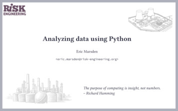
Analyzing data using PythonEric Marsden eric.marsden@risk-engineering.org The purpose of computing is insight, not numbers.– Richard Hamming

Where does this fit into risk engineering?datacurvefittingprobabilistic modelconsequence modelevent probabilitiesevent consequencesrisks

Where does this fit into risk engineering?datacurvefittingprobabilistic modelconsequence modelevent probabilitiesevent consequencescostsriskscriteriadecision-making

Where does this fit into risk engineering?datacurvefittingprobabilistic modelconsequence modelevent probabilitiesevent consequencesThese slidescostsriskscriteriadecision-making

Descriptive statistics

Descriptive statistics Descriptive statistics allow you to summarize information aboutobservations organize and simplify data to help understand it Inferential statistics use observations (data from a sample) to makeinferences about the total population generalize from a sample to a population

Descriptive statisticsSource: dilbert.com

Measures of central tendency Central tendency (the “middle” of your data) is measured either by themedian or the mean The median is the point in the distribution where half the values arelower, and half higher it’s the 0.5 quantile The (arithmetic) mean (also called the average or the mathematicalexpectation) is the “center of mass” of the distribution𝑏 continuous case: 𝔼(𝑋) 𝑎 𝑥𝑓 (𝑥)𝑑𝑥 discrete case: 𝔼(𝑋) 𝑖 𝑥𝑖 𝑃(𝑥𝑖 ) The mode is the element that occurs most frequently in your data

Illustration: fatigue life of aluminium sheetingMeasurements of fatigue life(thousands of cycles until rupture) ofstrips of 6061-T6 aluminium sheeting,subjected to loads of 21 000 PSI.Data from Birnbaum and Saunders(1958). import numpy cycles numpy.array([370, 1016, 1235, [.] 1560, 1792]) cycles.mean()1400.9108910891089 numpy.mean(cycles)1400.9108910891089 numpy.median(cycles)1416.0Source: Birnbaum, Z. W. and Saunders, S. C. (1958), A statistical model for life-length of materials, Journal of the American StatisticalAssociation, 53(281)

Aside: sensitivity to outliersNote: the mean is quite sensitive to outliers, the median much less. the median is what’s called a robust measure of central tendency import numpy weights numpy.random.normal(80, 10, 1000) numpy.mean(weights)79.83294314806949 numpy.median(weights)79.69717178759265 numpy.percentile(weights, 50)79.69717178759265 # 50th percentile 0.5 quantile median weights numpy.append(weights, [10001, 101010])# outliers numpy.mean(weights)190.4630171138418# -- big change numpy.median(weights)79.70768232050916# -- almost unchanged

Measures of central tendencyIf the distribution of data is symmetrical, then the meanis equal to the median.If the distribution is asymmetric (skewed), the mean isgenerally closer to the skew than the median.Degree of asymmetry is measured by skewness (Python:scipy.stats.skew())Negative skewPositive skew

Measures of variability Variance measures the dispersion (spread) of observations around themean 𝑉 𝑎𝑟(𝑋) 𝔼 [(𝑋 𝔼[𝑋])2 ] continuous case: 𝜎2 (𝑥 𝜇)2 𝑓 (𝑥)𝑑𝑥 where 𝑓 (𝑥) is the probability densityfunction of 𝑋 discrete case: 𝜎2 1𝑛 1𝑛 𝑖 1 (𝑥𝑖 𝜇)2 note: if observations are in metres, variance is measured in 𝑚2 Python: array.var() or numpy.var(array) Standard deviation is the square root of the variance it has the same units as the mean Python: array.std() or numpy.std(array)

Exercise: Simple descriptive statisticsTask: Choose randomly 1000 integers from a uniform distributionbetween 100 and 200. Calculate the mean, min, max, variance andstandard deviation of this sample. import numpy obs numpy.random.randint(100, 201, 1000) obs.mean()149.49199999999999 obs.min()100 obs.max()200 obs.var()823.99793599999998 obs.std()28.705364237368595

Histograms: plots of variabilityHistograms are a sort of bar graph that showsthe distribution of data values. The vertical axisdisplays raw counts or proportions.To build a histogram:123Subdivide the observations into several equalclasses or intervals (called “bins”)import matplotlib.pyplot as plt# our Birnbaum and Sanders failure dataplt.hist(cycles)plt.xlabel("Cycles until failure")25Count the number of observations in eachinterval20Plot the number of observations in eachinterval10Note: the width of the bins is important to obtain a“reasonable” histogram, but is subjective.155050010001500Cycles until failure20002500

Quartiles A quartile is the value that marks one of the divisionsthat breaks a dataset into four equal parts The first quartile, at the 25th percentile, divides thefirst ¼ of cases from the latter ¾ The second quartile, the median, divides the dataset inhalf The third quartile, the 75th percentile, divides the first¾ of cases from the latter ¼25% ofobservations25% of observations25% of observations25% of observations The interquartile range (IQR) is the distance betweenthe first and third quartiles 25th percentile and the 75th percentileinterquartile range

Box and whisker plot the median (horizontal line) lower and upper quartiles Q1 and Q3 (the box) upper whisker: last datum Q3 1.5 IQR the lower whisker: first datum Q1 - 1.5 IQR any data beyond the whiskers are typically calledoutliersimport matplotlib.pyplot as pltplt.boxplot(cycles)plt.xlabel("Cycles until failure")2500Cycles until failureA “box and whisker” plot or boxplot shows the spread ofthe data200015001000500plot whiskersNote that some peopleththe 5th and les for examples max valu1

Violin plotAdds a kernel density estimation to a boxplot250020001500import seaborn as sns1000sns.violinplot(cycles, orient "v")plt.xlabel("Cycles until failure")5000Cycles until failure

Bias and precisionPreciseImpreciseBiasedUnbiasedA good estimator should be unbiased, precise and consistent (converge as sample sizeincreases).

Estimating values In engineering, providing a point estimate is not enough: we also need toknow the associated uncertainty especially for risk engineering! One option is to report the standard error , where 𝜎̂ is the sample standard deviation (an estimator for the populationstandard deviation) and 𝑛 is the size of the sample𝜎̂ 𝑛 difficult to interpret without making assumptions about the distribution of theerror (often assumed to be normal) Alternatively, we might report a confidence interval

Confidence intervals A two-sided confidence interval is an interval [𝐿, 𝑈] such that C% of thetime, the parameter of interest will be included in that interval most commonly, 95% confidence intervals are used Confidence intervals are used to describe the uncertainty in a pointestimate a wider confidence interval means greater uncertainty

Interpreting confidence intervalspopulationmeanmmmmmmmmmmA 90% confidence interval means that 10% ofthe time, the parameter of interest will not beincluded in that interval.Here, for a two-sided confidence interval.

Interpreting confidence intervalspopulationmeanmmmA 90% confidence interval means that 10% ofthe time, the parameter of interest will not beincluded in that interval.mmmmHere, for a one-sided confidence interval.mmm

Illustration: fatigue life of aluminium sheetingConfidence intervals can be displayedgraphically on a barplot, as “error lines”.import seaborn as snssns.barplot(cycles, ci 95, capsize 0.1)plt.xlabel("Cycles until failure (95% CI)")Note however that this graphical presentationis ambiguous, because some authors representthe standard deviation on error bars. Thecaption should always state what the error barsrepresent.020040060080010001200Cycles until failure, with 95% confidence intervalData from Birnbaum and Saunders (1958)1400

Statistical inferencepopulationsampleStatistical inference means deducinginformation about a population byexamining only a subset of thepopulation (the sample).We use a sample statistic to estimatea population parameter.

How to determine the confidence interval? If you make assumptions about the distribution of your data (eg. “theobservations are normally distributed”), you can calculate the confidenceinterval for your estimation of the parameter of interest (eg. the mean)using analytical quantile measures If you don’t want to make too many assumptions, a technique called thebootstrap can help General idea: I want to determine how much uncertainty is generated by the fact that I onlyhave a limited sample of my full population If I had a “full” sample, I could extract a large number of limited samples andexamine the amount of variability in those samples (how much does myparameter of interest vary across these samples?) I only have a limited sample, but I can look at a large number of limitedsamples from my own limited sample, by sampling with replacement

Bootstrap methods “Bootstrapping” means resampling your data with replacement Instead of fitting your model to the original 𝑋 and 𝑦, you fit your model toresampled versions of 𝑋 and 𝑦 many times Provides 𝑛 slightly different models from which we create a confidenceinterval Hypothesis: observations are the result of a model plus noise

Bootstrapping confidence intervals in Python1Take a large number of samples of the same size as our original dataset, bysampling with replacement2For each sample, calculate the parameter of interest (eg. the mean)3Calculate the relevant percentile from the distribution of the parameter of interestdef bootstrap confidence intervals(data, estimator, percentiles, runs 1000):replicates numpy.empty(runs)for i in range(runs):replicates[i] estimator(numpy.random.choice(data, len(data), replace True))est numpy.mean(replicates)ci numpy.percentile(numpy.sort(replicates), percentiles)return (est, ci)

Illustration with ExcelImport your data into the firstrow of a spreadsheet (here wehave 10 observations).Calculate the sample mean (lastcolumn) using functionAVERAGE.

Illustration with ExcelThe first replicate, placed in therow under the sample, isobtained by resampling withreplacement from the originalsample.Each cell contains the formulaINDEX(A1:J1,RANDBETWEEN(1, 10)),meaning “choose a randomelement from the first row”.Calculate the mean of the firstreplicate (last column) usingfunction AVERAGE.

Illustration with ExcelGenerate a large number ofreplicates (here 18), in successiverows of the spreadsheet.The mean of all the replicatemeans (here in bold) is thebootstrapped mean. Otherestimations such as confidenceintervals can be obtained fromthe blue column of replicatemeans.

Illustration: bootstrapped mean of Birnbaum dataLet’s calculate the bootstrapped mean and associated 95% confidence interval forthe Birnbaum and Saunders (1958) fatigue data. import numpy cycles numpy.array([370, 1016, 1235, [.] 1560, 1792]) cycles.mean()1400.9108910891089 est, ci bootstrap confidence intervals(cycles, numpy.mean, [5, 95]) print("Bootstrapped mean and CI: {:.1f} [{:.1f}, {:.1f}]".format(est, ci[0], ci[1]))Bootstrapped mean and CI95: 1403.7 [1332.8, 1478.9]

Fitting models

Fitting a distribution to observations The probability distributions defined in scipy.stats have a fit()method to find the parameters that provide a “best” fit more precisely, the maximum likelihood of being the best fit For example scipy.stats.norm.fit(data) scipy.stats.lognorm.fit(data) scipy.stats.expon.fit(data) scipy.stats.pareto.fit(data) They return different parameters depending on the distribution, withsome common parameters loc for the mean scale for the standard deviation