Transcription
Hierarchical Linear ModelsJoseph Stevens, Ph.D., University of Oregon(541) 346-2445, stevensj@uoregon.edu Stevens, 20071
Overview and resources OverviewWeb site and links: www.uoregon.edu/ stevensj/HLMSoftware: HLMMLwinNMplusSASR and S-PlusWinBugs2
Workshop Overview Preparing dataTwo Level modelsTesting nested hierarchies of modelsEstimationInterpreting resultsThree level modelsLongitudinal modelsPower in multilevel models3
Hierarchical Data StructuresMany social and natural phenomena have a nested orclustered organization: Children within classrooms within schools Patients in a medical study grouped within doctorswithin different clinics Children within families within communities Employees within departments within businesslocations4
GroupingGrouping andand membershipmembership inin particularparticularunitsunits andand clustersclusters areare importantimportant
Hierarchical Data StructuresMore examples of nested or clustered organization: Children within peer groups within neighborhoods Respondents within interviewers or raters Effect sizes within studies within methods (metaanalysis) Multistage sampling Time of measurement within persons withinorganizations6
Simpson’s Paradox:Clustering Is ImportantWell known paradox in which performance of individualgroups is reversed when the groups are combinedQuiz 1Quiz 2TotalGina60.0%10.0%55.5%Sam90.0%30.0%35.5%Quiz 1Quiz 2TotalGina60 / 1001 / 1061 / 110Sam9 / 1030 / 10039 / 1107
Simpson’s Paradox: Other Examples20062006 USUS SchoolSchool xbiascase: Inpastresearch,privateIn past research, private schoolsschools achieveachieve higherhigher thanthan publicpublicschools UCBsuedschoolsUCBsued forfor biasbias byby womenwomen applyingapplying toto gradgrad schoolschoolwastoadditionalsupporttheStudywas expectedexpectedto provideprovideadditionalsupporttothe ideaidea thatthat igures showedshowedmenmore likelylikelyto terschoolsperformbetter and“WhentheOakiesleftOklahomaandmovedto Whenanalyzedbyindividualdepartment,turnedoutthatno isedtheIQofbothstates.”USEDstudy(using itmultilevelCalifornia,raised amodeling):theIQ of both rtmentshoweda bias;bias;––forWillRogers sWomenappliedtolowadmissionratedepartments Women applied to low admission rate departments ertakingdemographicgroupinginto account,account, therethere waswas ference betweenbetween publicpublic andand privateprivate andand differencesdifferences werewerealmostalmost equallyequally splitsplit inin favorfavor ofof eacheach schoolschool typetype8
HypotheticalHypothetical DataData ExampleExample fromfrom SnijdersSnijders &&BoskerBosker (1999),(1999), nn 2,2, j 5,j 5, njnj NN 1010Participant (i)Cluster (j)Outcome (Y)Predictor (X)11512173324142645333635574248446951510537
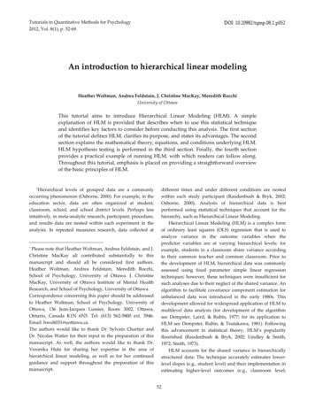
AllAll 1010 casescases analyzedanalyzed withoutwithout takingtaking clustercluster membershipmembership intointo account:account:Model SummaryModel1R.333aR Square.111AdjustedR Square.000Std. Error ofthe Estimate1.826a. Predictors: (Constant), icientsBStd. ta-.333t3.671-1.000Sig.006.347a. Dependent Variable: YY 5.333 -.333(X) rInterpretation: There’s a negative relationshipbetween the predictor X and the outcome Y, aone unit increase in X results in .333 lower Y
YY 5.3335.333 -.333(X)-.333(X) rr87β06Y543β1210012345678XThis is an example of a disaggregated analysis
AnotherAnother alternativealternative isis toto analyzeanalyzedatadata atat thethe aggregatedaggregated groupgroup levellevelParticipant(i)Cluster 4248446951510537Cluster (j)Outcome (Y)Predictor (X)162253344435526
TheThe clustersclusters areare analyzedanalyzed withoutwithout takingtaking individualsindividuals intointo account:account:Model SummaryModel1R1.000aR Square1.000AdjustedR Square1.000Std. Error ofthe Estimate.000a. Predictors: (Constant), zedCoefficientsBStd. ta-1.000tSig.a. Dependent Variable: MEANYY 8.000 -1.000(X) rInterpretation: There’s a negative relationshipbetween the predictor X and the outcome Y, aone unit increase in X results in 1.0 lower Y
This is an example of a disaggregated analysisY 8.000 -1.000(X) rβ087MEAN Y654β132101234MEAN X567
A third possibility is to analyze each cluster separately,looking at the regression relationship within each group876Y5432100123456XYij Yj 1.00(X ij X j ) rij78
MultilevelMultilevel regressionregression takestakes bothboth levelslevels intointo account:account:Y 8.000 -1.000(X) rYij Yj 1.00( X ij X j ) rijYij 8.00 1.00( X j ) 1.00(X ij X j ) rij
TakingTaking thethe multilevelmultilevel structurestructure ofof thethe datadata intointo account:account:Within groupregressions8Between Groups Regression76Y5432Total Regression1001234X5678
Why Is Multilevel Analysis Needed? Nesting creates dependencies in the data Dependencies violate the assumptions of traditionalstatistical models (“independence of error”, “homogeneityof regression slopes”)Dependencies result in inaccurate statistical estimatesImportant to understand variation at differentlevels18
Decisions About Multilevel Analysis Properly modeling multilevel structure oftenmatters (and sometimes a lot)Partitioning variance at different levels is useful22 tau and sigma (σ Y τ σ ) policy & practice implicationsCorrect coefficients and unbiased standard errors“Randomization by cluster accompanied by analysis Cross-levelinteraction by individual is an exercise inappropriateto randomization Understandingand modelingsite or(Cornfield,cluster 1978,self-deceptionand shouldbe discouraged”variabilitypp.101-2) 19
Preparing Data for HLM Analysis Use of SPSS as a precursor to HLM assumedHLM requires a different data file for each level in the HLManalysisPrepare data first in SPSS Clean and screen data Treat missing data ID variables needed to link levels Sort cases on IDThen import files into HLM to create an “.mdm” file20
Creating an MDM file Example: Go to “Examples” folder and then “Appendix A” in theHLM directoryOpen “HSB1.sav” and “HSB2.sav”21
Start HLM and choose “Make newMDM file” from menu; followedby “Stat package input”
For a two level HLM model staywith the default “HLM2”
Click “Browse”, identify thelevel 1 data file and open it
Check off the ID linkingvariable and all variables toClick on “Choose Variables”be included in the MDM file
Provide a name for the MDM fileClick on “Save mdmt file” and(use .mdm as the suffix)supply a name for the syntaxcommand file
Results will briefly appearClick on “Make MDM”
Click on “ChecktoTheStats”click “Done”see, save, or print results
You should see a screen likethis. You can now begin tospecify your HLM model
Two-Level HLM Models30
The Single-Level, Fixed Effects RegressionModelYi β0 β1X1i β2X2i βkXki ri The parameters βkj are considered fixed One for all and all for oneSame values for all i and j; the single level modelThe ri ’s are random: ri N(0, σ) andindependent31
The Multilevel Model Takes groups into account and explicitly modelsgroup effectsHow to conceptualize and model group levelvariation?How do groups vary on the model parameters?Fixed versus random effects32
Fixed vs. Random Effects Fixed Effects represent discrete, purposefully selected orexisting values of a variable or factor Fixed effects exert constant impact on DVRandom variability only occurs as a within subjects effect (level 1)Can only generalize to particular values usedRandom Effects represent more continuous or randomlysampled values of a variable or factor Random effects exert variable impact on DVVariability occurs at level 1 and level 2Can study and model variabilityCan generalize to population of values33
Fixed vs. Random Effects? Use fixed effects if The groups are regarded as unique entitiesIf group values are determined by researcher throughdesign or manipulationSmall j ( 10); improves powerUse random effects if Groups regarded as a sample from a larger populationResearcher wishes to test effects of group level variablesResearcher wishes to understand group level differencesSmall j ( 10); improves estimation34
Fixed Intercepts Model The simplest HLM model is equivalent to a oneway ANOVA with fixed effects:Yij γ00 rij This model simply estimates the grand mean (γ00)and deviations from the grand mean (rij)Presented here simply to demonstrate control offixed and random effects on all parameters35
Note the equation has no “u” residualterm; this creates a fixed effect model36
37
ANOVA Model (random intercepts) Note theof u0jvaryingallowsA simple HLM modelwithadditionrandomlydifferent intercepts for each j unit, ainterceptsrandom effects modelEquivalent to a one-way ANOVA with randomeffects:Yij β0j rijβ0j γ00 u0jYij γ00 u0j rij38
39
40
ANOVA Model In addition to providing parameter estimates, theANOVA model provides information about thepresence of level 2 variance (the ICC) and whetherthere are significant differences between level 2unitsThis model also called the Unconditional Model(because it is not “conditioned” by any predictors)and the “empty” modelOften used as a baseline model for comparison tomore complex models41
Variables in HLM Models Outcome variablesPredictors Control variables Explanatory variablesVariables at higher levels Aggregated variables (Is n sufficient forrepresentation?) Contextual variables42
Conditional Models: ANCOVA Adding a predictor to the ANOVA model results in anANCOVA model with random intercepts:Yij β0j β1(X1) rijβ0j γ00 u0jβ1 γ10 Note that the effect of X is constrained to be the samefixed effect for every j unit (homogeneity of regressionslopes)43
44
45
Conditional Models: Random Coefficients An additional parameter results in random variationof the slopes:Yij β0j β1(X1) rijβ0j γ00 u0jβ1j γ10 u1j Both intercepts and slopes now vary from group togroup46
47
48
Standardized coefficientsStandardized coefficient at level 1:β0j (SDX / SDY)Standardized coefficient at level 2:γ00 (SDX / SDY)49
Modeling variation at Level 2:Intercepts as OutcomesYij β0j β1jX1ij rijβ0j γ00 γ0jWj u0jβ1j γ10 u1j Predictors (W’s) at level 2 are used to modelvariation in intercepts between the j units50
Modeling Variation at Level 2: Slopes asOutcomesYij β0j β1jX1ij rijβ0j γ00 γ0jWj u0jβ1j γ10 γ1jWj u1j Do slopes vary from one j unit to another?W’s can be used to predict variation in slopes as well51
Variance Components Analysis VCA allows estimation of the size of randomvariance components Important issue when unbalanced designs areused Iterative procedures must be used (usually MLestimation)Allows significance testing of whether there isvariation in the components across units52
Estimating Variance Components:Unconditional ModelVar(Yij) Var(u0j) Var(rij) τ0 σ253
HLM OutputFinal estimation of variance ---------Random EffectStandardVariancedf Chi-square P-valueDeviation -------INTRCPT1,U014.38267 206.86106 14 457.32201 0.000level-1,R32.58453 --------Statistics for current covariance components ----Deviance 21940.853702Number of estimated parameters 254
Variance explainedR2 at level 1 1 – (σ2cond τcond) / (σ2uncond τuncond)R2 at level 2 1 – [(σ2cond / nh) τcond] / [(σ2uncond / nh) τuncond]Where nh the harmonic mean of n for the level 2 units(k / [1/n1 1/n2 1/nk])55
Comparing models Deviance tests Under “Other Settings” on HLM tool bar, choose“hypothesis testing”Enter deviance and number of parameters from baselinemodelVariance explained Examine reduction in unconditional model variance aspredictors added, a simpler level 2 formula:R2 (τ baseline – τ conditional) / τ baseline56
57
Deviance Test ResultsStatistics for current covariance components --------------Deviance 21615.283709Number of estimated parameters 2Variance-Covariance components -------------Chi-square statistic 325.56999Number of degrees of freedom 0P-value .50058
Testing a Nested Sequence of HLMModels1. Test unconditional model2. Add level 1 predictors Determine if there is variation across groupsIf not, fix parameterDecide whether to drop nonsignificant predictorsTest deviance, compute R2 if so desired3. Add level 2 predictors Evaluate for significanceTest deviance, compute R2 if so desired59
Example Use the HSB MDM file previously created topractice running HLM models: UnconditionalLevel 1 predictor fixed, then randomLevel 2 predictor60
Statistical Estimation in HLM Models Estimation Methods Parameter estimation FMLRMLEmpirical Bayes estimationCoefficients and standard errorsVariance ComponentsParameter reliabilityCenteringResidual files61
Estimation Methods: Maximum LikelihoodEstimation (MLE) Methods MLE estimates model parameters by estimating aset of population parameters that maximize alikelihood functionThe likelihood function provides the probabilitiesof observing the sample data given particularparameter estimatesMLE methods produce parameters that maximizethe probability of finding the observed sample data62
Estimation MethodsRMLRML –– RestrictedRestricted MaximumMaximum Likelihood,Likelihood, onlyonlyFML–– FullMaximumtheareinFMLFullcomponentsMaximum Likelihood,Likelihood,boththe regressionregressionthe variancevariancecomponentsare includedincludedbothin yestimates the Full:thelikelihoodfunctionFull: thelikelihoodfunctionfixed effects and then the variancefixed effects and then the s)CheckCheckononsoftwaresoftwaredefaultdefault63
Estimation Methods RML expected to lead to better estimates especially whenj is smallFML has two advantages: Computationally easier With FML, overall chi-square tests both regressioncoefficients and variance components, with RML onlyvariance components are tested Therefore if fixed portion of two models differ, mustuse FML for nested deviance tests64
Computational Algorithms Several algorithms exist for existing HLM models: Expectation-Maximization (EM)Fisher scoringIterative Generalized Least Squares (IGLS)Restricted IGLS (RIGLS)All are iterative search and evaluation procedures65
Model Estimation Iterative estimation methods usually begin with aset of start valuesStart values are tentative values for the parametersin the model Program begins with starting values (usuallybased on OLS regression at level 1) Resulting parameter estimates are used as initialvalues for estimating the HLM model66
Model Estimation Start values are used to solve model equations on firstiterationThis solution is used to compute initial model fitNext iteration involves search for better parameter valuesNew values evaluated for fit, then a new set of parametervalues triedWhen additional changes produce no appreciableimprovement, iteration process terminates (convergence)Note that convergence and model fit are very different issues67
IntermissionIntermission
Centering No centering (common practice in single levelregression)Centering around the group mean ( X j )Centering around the grand mean (M )A known population meanA specific meaningful time point69
Centering: The Original Metric Sensible when 0 is a meaningful point on theoriginal scale of the predictor For example, amount of training ranging from 0to 14 days Dosage of a drug where 0 represents placebo orno treatmentNot sensible or interpretable in many othercontexts, i.e. SAT scores (which range from 200 to800)70
01020304050β 0 j E (Yij X ij 0)71
Centering Around the Grand Mean Predictors at level 1 (X’s) are expressed as deviationsfrom the grand mean (M): (Xij – M)Intercept now expresses the expected outcome value (Y)for someone whose value on predictor X is the same asthe grand mean on that predictorCentering is computationally more efficientIntercept represents the group mean adjusted for thegrand mean X j- MVariance of β0j τ00, the variance among the level-2 unitmeans adjusted for the grand mean72
Centering Around the Grand Meanβ01β02β0301020304050β 0 j E (Yij X ij γ 00 )73
Centering Around the Group Mean Individual scores are interpreted relative to their group mean ( X ij X )The individual deviation scores are orthogonal to the group meansIntercept represents the unadjusted mean achievement for thegroupUnbiased estimates of within-group effectsMay be necessary in random coefficient models if level 1 predictoraffects the outcome at both level 1 and level 2Can control for unmeasured between group differencesBut can mask between group effects; interpretation is morecomplex74
Centering Around the Group Mean Level 1 results are relative to group membership Intercept becomes the unadjusted mean for group j Should include level 2 mean of level 1 variables to fullydisentangle individual and compositional effects Variance β0j is now the variance among the level 2 unitmeans75
Centering Around the Group MeanIf X1 25, then β 01 E (Yi1 X i1 25)If X 2 20, then β 02 E (Yi 2 X i 2 20)If X 3 18, then β 03 E (Yi 3 X i 3 18)0102030405076
Parameter estimation Coefficients and standard errors estimated throughmaximum likelihood procedures (usually) The ratio of the parameter to its standard error produces a Wald testevaluated through comparison to the normal distribution (z)In HLM software, a more conservative approach is used: t-tests are used for significance testingt-tests more accurate for fixed effects, small n, and nonnormaldistributions)Standard errorsVariance components77
Parameter reliability Analogous to score reliability: ratio of true score variance tototal variance (true score error)In HLM, ratio of true parameter variance to total variabilityVarianceof error of
Preparing Data for HLM Analysis Use of SPSS as a precursor to HLM assumed HLM requires a different data file for each level in the HLM analysis Prepare data first in SPSS Clean and screen data Treat mis