Transcription
Generalized Linear Mixed Models(illustrated with R on Bresnan et al.’s datives data)Christopher Manning23 November 2007In this handout, I present the logistic model with fixed and random effects, a form of Generalized LinearMixed Model (GLMM). I illustrate this with an analysis of Bresnan et al. (2005)’s dative data (the versionsupplied with the languageR library). I deliberately attempt this as an independent analysis. It is animportant test to see to what extent two independent analysts will come up with the same analysis of a setof data. Sometimes the data speaks so clearly that anyone sensible would arrive at the same analysis. Often,that is not the case. It also presents an opportunity to review some exploratory data analysis techniques, aswe start with a new data set. Often a lot of the difficulty comes in how to approach a data set and to definea model over which variables, perhaps transformed.1Motivating GLMMsI briefly summarize the motivations for GLMMs (in linguistic modeling): The Language-as-fixed-effect-fallacy (Clark 1973 following Coleman 1964). If you want to make statements about a population but you are presenting a study of a fixed sample of items, then you cannotlegitimately treat the items as a fixed effect (regardless of whether the identity of the item is a factorin the model or not) unless they are the whole population.– Extension: Your sample of items should be a random sample from the population about whichclaims are to be made. (Often, in practice, there are sampling biases, as Bresnan has discussedfor linguistics in some of her recent work. This can invalidate any results.) Ignoring the random effect (as is traditional in psycholinguistics) is wrong. Because the often significantcorrelation between data coming from one speaker or experimental item is not modeled, the standarderror estimates, and hence significances are invalid. Any conclusion may only be true of your randomsample of items, and not of another random sample. Modeling random effects as fixed effects is not only conceptually wrong, but often makes it impossibleto derive conclusions about fixed effects because (without regularization) unlimited variation can beattributed to a subject or item. Modeling these variables as random effects effectively limits how muchvariation is attributed to them (there is an assumed normal distribution on random effects). For categorical response variables in experimental situations with random effects, you would like tohave the best of both worlds: the random effects modeling of ANOVA and the appropriate modelingof categorical response variables that you get from logistic regression. GLMMs let you have bothsimultaneously (Jaeger 2007). More specifically:– A plain ANOVA is inappropriate with a categorical response variable. The model assumptionsare violated (variance is heteroscedastic, whereas ANOVA assumes homoscedasticity). This leadsto invalid results (spurious null results and significances).1
– An ANOVA can perform poorly even if transformations of the response are performed. At anyrate, there is no reason to use this technique: cheap computing makes use of a transformedANOVA unnecessary.– A GLMM gives you all the advantages of a logistic regression model:1 Handles a multinomial response variable.Handles unbalanced dataGives more information on the size and direction of effectsHas an explicit model structure, adaptable post hoc for different analyses (rather than requiring different experimental designs) Can do just one combined analysis with all random effects in it at once. Technical statistical advantages (Baayen, Davidson, and Bates). Maybe mainly incomprehensible, butyou can trust that worthy people think the enterprise worthy.– Traditional methods have deficiencies in power (you fail to demonstrate a result that you shouldbe able to demonstrate)– GLMMs can robustly handle missing data, while traditional methods cannot.– ? GLMMs improve on disparate methods for treating continuous and categorical responses ?.[I never quite figured out what this one meant – maybe that working out ANOVA models andtractable approximations for different cases is tricky, difficult stuff?]– You can avoid unprincipled methods of modeling heteroscedasticity and non-spherical error variance.– It is practical to use crossed rather than nested random effects designs, which are usually moreappropriate– You can actually empirically test whether a model requires random effects or not. But in practice the answer is usually yes, so the traditional ANOVA practice of assuming yesis not really wrong.– GLMMs are parsimonious in using parameters, allowing you to keep degrees of freedom (givingsome of the good effects listed above). The model only estimates a variance for each randomeffect.2Exploratory Data Analysis (EDA)First load the data (I assume you have installed the languageR package already). We will use the dativedata set, which we load with the data function. Typing dative at the command line would dump it to yourwindow, but that isn’t very useful for large data sets. You can instead get a summary: library(languageR) data(dative) summary(dative)SpeakerModalityS1104 : 40spoken :2360S1083 : 30written: 903S1151 : 30S1139 : 29givepaysellsendVerb:1666: 207: 206: 172SemanticClassa:1433c: 405f: 59p: 228LengthOfRecipientAnimacyOfRecMin.: 1.000animate :30241st Qu.: 1.000inanimate: 239Median : 1.000Mean: 1.8421 Jaeger’s suggesting that GLMMs give you the advantage of penalized likelihood models is specious; similar regularizationmethods have been developed and are now widely used for every type of regression analysis, and ANOVA is equivalent to atype of linear regression analysis, as Jaeger notes.2
S1019 : 28(Other):2203NA’s: 903DefinOfRecdefinite :2775indefinite: pronominal:2034169t:1138128715LengthOfThemeMin.: 1.0001st Qu.: 2.000Median : 3.000Mean: 4.2723rd Qu.: 5.000Max.:46.0003rd Qu.: 2.000Max.:31.000AnimacyOfThemeDefinOfThemeanimate : 74definite : 929inanimate:3189indefinite:2334PronomOfTheme 2 NP:2414accessible: 615pronominal: 421PP: 849given:2302new: 346AccessOfThemeaccessible:1742given: 502new:1019Much more useful!In terms of the discussion in the logistic regresssion handout, this is long form data – each observed datapoint is a row. Though note that in a case like this with many explanatory variables, the data wouldn’tactually get shorter if presented as summary statistics, because the number of potential cells (# speakers # Modality # Verb . . . ) well exceeds the observed number of data items. The data has also all beenset up right, with categorical variables made into factors etc. If you are starting from data read in from atab-separated text file, that’s often the first thing to do.If you’ve created a data set, you might know it intimately. Otherwise, it’s always a good idea to get agood intuitive understanding of what is there. The response variable is RealizationOfRecipient (long variablenames, here!). Note the very worrying fact that over half the tokens in the data are instances of the verbgive. If it’s behavior is atypical relative to ditransitive verbs, that will skew everything. Under, Speaker,NA is R’s special “not available” value for missing data. Unavailable data attributes are very common inpractice, but often introduce extra statistical issues (and you often have to be careful to check how R ishandling the missing values). Here, we guess from the matching 903’s that all the written data doesn’t havethe Speaker listed. Since we’re interested in a mixed effects model with Speaker as a random effect, we’llwork with just the spoken portion (which is the Switchboard data).spdative - subset(dative, Modality "spoken")You should look at the summary again, and see how it has changed. It has changed a bit (almost all thepronominal recipients are in the spoken data, while most of the nonpronominal recipients are in the writtendata; nearly all the animate themes are in the spoken data). It’s also good just to look at a few rows (notethat you need that final comma in the array selector!): spdative[1:5,]Speaker Modality Verb SemanticClass LengthOfRecipient AnimacyOfRec DefinOfRec903S1176spoken givea1inanimatedefinite904S1110spoken givec2animate indefinite905S1110spoken paya1animatedefinite906S1146spoken givea2animatedefinite907S1146spoken givet2animatedefinitePronomOfRec LengthOfTheme AnimacyOfTheme DefinOfTheme PronomOfTheme903pronominal2inanimateindefinite nonpronominal904 inal1inanimateindefinite nonpronominal906 nonpronominal4inanimateindefinite nonpronominal907 nonpronominal3inanimatedefinite nonpronominal3
Figure 1: Mosaic plot. Most data instances are animate recipient, inanimate theme, realized as an nt AccessOfRec essibleNP accessiblenewPP accessibleaccessibleCategorical predictorsDoing exploratory data analysis of categorical variables is harder than for numeric variables. But it’s certainlyuseful to look at crosstabs (even though, as discussed, you should trust regression outputs not the marginalsof crosstabs for what factors are important). But they give you a sense of the data, and having done this willat least allow you to notice when you make a mistake in model building and the predictions of the modelproduced are clearly not right. For just a couple of variables, you can also graph them with a mosaicplot. Butthat quickly becomes unreadable for too many variables at once. . . . Figure 1 already isn’t that informativeto me beyond the crosstabs. I concluded that a majority of the data instances have inanimate theme andanimate recipient, and these are overwhelmingly realized as a ditransitive (NP recipient). spdative.xtabs - xtabs( RealizationOfRecipient AnimacyOfRec AnimacyOfTheme) spdative.xtabs, , AnimacyOfTheme animateAnimacyOfRecRealizationOfRecipient animate inanimateNP170PP4654
, , AnimacyOfTheme inanimateAnimacyOfRecRealizationOfRecipient animate inanimateNP176181PP37872 mosaicplot(spdative.xtabs, color T)These methods should be continued looking at various of the other predictors in natural groups. The responseis very skewed: 1859/(1859 501) 78.8% of the examples are NP realization (ditransitives). Looking atother predictors, most of the data is also indefinite theme and definite recipient, realized as an NP. Andmost of the data is nonpronominal theme and pronominal recipient which is overwhelmingly realized as anNP. With slightly less skew, much of the data has anaccessible theme and a given recipient, usually realizedas an NP. For semantic class, “t” stands out as preferring PP realization of the theme (see Bresnan et al.(2005, p. 12) on these semantic classes – “t” is transfer of possession). Class “p” (prevention of possession)really seems to prefer NP realization. Finally, we might check whether give does on average behave like otherverbs. The straight marginal looks okay (if probably not passing a test for independence). A crosstab alsoincluding PronomOfRec looks more worrying: slightly over half of instances of give with a nonpronominalrecipient NP are nevertheless ditransitive, whereas less than one third over such cases with other verbs haveNP realization. Of course, there may be other factors which explain this, which a regression analysis cantease out. xtabs( RealizationOfRecipient I(Verb "give"))I(Verb "give")RealizationOfRecipient FALSE TRUENP776 1083PP321 180 xtabs( RealizationOfRecipient I(Verb "give") PronomOfRec), , PronomOfRec nonpronominalI(Verb "give")RealizationOfRecipient FALSE TRUENP83 109PP18598, , PronomOfRec pronominalI(Verb "give")RealizationOfRecipient FALSE TRUENP693 974PP13682It can also be useful to do crosstabs without the response variable. An obvious question is how pronominality, definiteness, and animacy interrelate. I put a couple of mosaic plots for this in Figure 2. Theirdistribution is highly skewed and strongly correlated.22.2Numerical predictorsThere are some numeric variables (integers, not real numbers): the two lengths. If we remember the Wasowpaper and Hawkins’s work, we might immediately also wonder where the difference between these two2 These two were drawn with the mosaic() function in the vcd package, which has extra tools for visualizing categorical data.This clearly seems to have been what Baayen actually used to draw his Figure 2.6 (p. 36) and not mosaicplot(), despite whatis said on p. 35.5
RecipientDefinOfRecdefinitepronominalnonpronominal re 2: Interaction of definiteness, animacy, and pronominalitylengths might be an even better predictor, so we’ll add it to the data frame. Thinking ahead to transformingexplanatory variables, it also seems useful to have the ratio of the two lengths. We’ll add these variablesbefore we attach to the data frame, so that they will be available.3 spdative - transform(spdative, LengthOfThemeMinusRecipient LengthOfTheme - LengthOfRecipient) spdative - transform(spdative, RatioOfLengthsThemeOverRecipient LengthOfTheme / LengthOfRecipient) attach(spdative)If we’re fitting a logistic model, we might check whether a logistic model works for these numeric variables.Does a unit change in length cause a constant change in the log odds. We could plot with untransformedvalues, looking for a logistic curve, but it is usually better to plot against logit values and to check againsta straight line. We’ll do both. First we examine the data with crosstabs: xtabs( RealizationOfRecipient cipient123456NP 1687 13319844PP 228 1396124128 xtabs( RealizationOfRecipient LengthOfTheme)LengthOfThemeRealizationOfRecipient 12345678NP 358 515 297 193 145 77 75 46PP 268 116 42 22 16 1434LengthOfThemeRealizationOfRecipient 17 18 19 21 23 24 25 We could directly use length as an integer in our plot, but it gets hopelessly sparse for big lengths (P (NP realization) 0.33 for length 9 but 0 for length 8 or 10. . . ). So we will group using the cut command. This defines a factorby categoricalizing a numeric variable into ranges, but I’m going to preserve and use the numeric values inmy plot. I hand chose the cut divisions to put a reasonable amount of data into each bin. Given the integernature of most of the data, hand-done cuts seemed more sensible than cutting it automatically. (The output3 Of course, in reality, I didn’t do this. I only thought to add these variables later in the analysis. I then added them as here,and did an attach again. It complains about hiding the old variables, but all works fine.6
of the cut command is a 2360 element vector mapping the lengths onto ranges. So I don’t print it out here!)The table command then produces a crosstab (like xtabs, but not using the model syntax), and prop.tablethen turns the counts into a proportion of a table by row, from which we take the first column (recipientNP realization proportion). divs - c(0,1,2,3,4,5,6,10,100)divs2 - c(-40,-6,-4,-3,-2,-1,0,1,2,3,4,6,40)divs3 - p.leng.group - cut(LengthOfRecipient, divs)theme.leng.group - cut(LengthOfTheme, divs)theme.minus.recip.group - cut(LengthOfThemeMinusRecipient, divs2)log.theme.over.recip.group - cut(log(RatioOfLengthsThemeOverRecipient), divs3)recip.leng.table - table(recip.leng.group, OfRecipientrecip.leng.groupNPPP(0,1]1687 228(1,2]133 0]16 theme.leng.table - table(theme.leng.group, RealizationOfRecipient) theme.minus.recip.table - table(theme.minus.recip.group, RealizationOfRecipient) log.theme.over.recip.table - table(log.theme.over.recip.group, RealizationOfRecipient) rel.freq.NP.recip.leng - prop.table(recip.leng.table, 1)[,1] 6](6,10] (10,100]0.8809399 0.4889706 0.2375000 0.2500000 0.2500000 0.3333333 0.1153846 0.1428571 rel.freq.NP.theme.leng - prop.table(theme.leng.table, 1)[,1] rel.freq.NP.theme.minus.recip - prop.table(theme.minus.recip.table, 1)[,1] rel.freq.NP.log.theme.over.recip - prop.table(log.theme.over.recip.table, 1)[,1]That’s a lot of setup! Doing EDA can be hard work. But now we can actually plot numeric predictorsagainst the response variable and fit linear models to see how well they correlate. It sticks out in the datathat most themes and recipients are quite short, but occasional ones can get very long. The data cries outfor some sort of data transform. sqrt() and log() are the two obvious data transforms that should come tomind when you want to transform data with this sort of distribution (with log() perhaps more natural here).We can try them out. We plot each of the raw and log and sqrt transformed values of each of theme andrecipient length against each of a raw probability of NP realization and the logit of that quantity, giving 12plots and 12 regressions. Then I make 4 more plots by considering the difference between their lengths andthe log of the ratio between their lengths against both the probability and the logit, giving 16 plots in total.Looking ahead to using a log() transform was why I defined the ratio of lengths – since I can’t apply log()to 0 or negative numbers, but it is completely sensible to apply it to a ratio. In fact, there is every reasonto think that this might be a good explanatory factor.This gives a fairly voluminous amount of commands and output to wade through, so I will display thegraphical results in Figure 3, and put all the calculation details in an appendix. But you’ll need to look atthe calculation details to see what I did to produce the figure.I made the regression lines by simply making linear models. I define a center for each factor, which is amixture of calculation and sometimes just a reasonable guess for the extreme values. Then I fit regressionlines by ordinary linear regression not logistic regression. So model fit is assessed by squared error (which7
.50.60.21.552.02.5103.03.5 101leng.centers32.51.52.02.50.50 1 2 20.00.51.01.52.02.5Logit sqrt(Recip Length)R2 0.6761.01.52.02.53.03.5sqrt(leng.centers)R2 0.827Prob log(Theme/Recip) 21.5log(leng.centers)Prob sqrt(Recip Length)R2 0.6471.01.0Logit log(Recip Length)R2 0.804sqrt(leng.centers)R2 0.765 50.5log(leng.centers)Logit Theme Recip .freq.NP.recip.leng)122.51.5 3 rs2101.51.00.0log(leng.centers)R2 0.788sqrt(leng.centers)0.608Logit sqrt(Theme Length)R2 0.5930.5logit(rel.freq.NP.theme.leng)2.52.5Prob log(Recip Length)leng.centersProb Theme RecipR2 0.706 562.00 1 241.50.20 1 2 221.0log(leng.centers)Logit Recip LengthR2 0.544sqrt(leng.centers) 100.5 req.NP.recip.leng)10R2 0.5191.5122328Prob sqrt(Theme 0.60.2rel.freq.NP.recip.lengR2 ure 3: Assessing the numeric predictors.Prob Recip Length26leng.centersR2 0.885040.602.51.52Logit log(Theme Length)R2 0.736Logit log(Theme/Recip) 212Prob log(Theme Length)R2 ver.recip2Logit Theme LengthR2 0.4540.5R2 .NP.theme.lengProb Theme Length 2 101leng.centers323
ignores the counts supporting each cell), not logistic model likelihood. This is sort of wrong, but it seemsnear enough for this level of EDA, and avoids having to do more setup. . . . This isn’t the final model, we’rejust trying to see how the data works. Note also that for plot() you specify x first then y, whereas in modelbuilding, you specify the response variable y first. . . . I was careful to define the extreme bins as wide enoughto avoid any categorical bins (so I don’t get infinite logits).Having spent 2 hours producing Figure 3, what have I learned? For both theme length and recipient length, I get better linear fit by using a logit response variablethan a probability, no matter what else I do. That’s good for a logit link function, which we’ll be using. For both theme length and recipient length, for both probabilities and logits, using raw length worksworst, sqrt is in the middle, and log scaling is best. Recipient length is more predictive of the response variable than theme length. Log transformedrecipient length has an R2 of 0.80 with the logit of the response variable. The difference between lengths between theme and recipient works noticeably better than either usedas a raw predictor. But it isn’t better than those lengths log transformed, and we cannot log transforma length difference. Incidentally, although the graph in the bottom right looks much more like a logistic S curve thananything we have seen so far, it seems like it isn’t actually a logistic S but too curvy. That is, plottedagainst the logit scale in the next graph, it still doesn’t become a particularly straight line. (Thisactually surprised me at first, and I thought I’d made a mistake, but it seems to be correct.) Using log(LengthOfTheme/LengthOfRecipient) really works rather nicely, and has R2 0.89. Thisseems a good place to start with a model!3Building GLMMsThere are essentially two ways to proceed: starting with a small model and building up or starting with abig model and trimming down. Many prefer the latter. Either can be done automatically or by hand. Ingeneral, I’ve been doing things by hand. Maybe I’m a luddite, but I think you pay more attention that way.Model building is still an art. It also means that you build an order of magnitude less models. Agresti (2002,p. 211) summarizes the model building goal as follows: “The model should be complex enough to fit thedata well. On the other hand, it should be simple to interpret, smoothing rather than overfitting the data.”The second half shouldn’t be forgotten.For the spoken datives data, the two random effects are Speaker and Verb. Everything else is a fixedeffect (except the response variable, and Modality, which I ignore – I should really have dropped it fromthe data frame). Let’s build a model of this using the raw variables as main effects. You use the lmer()function in the lme4 library, and to get a logistic mixed model (not a regular linear mixed model), you mustspecify the family ”binomial” parameter. Random effects are described using terms in parentheses using apipe ( ) symbol. I’ve just put in a random intercept term for Speaker and Verb. In general this seems tobe sufficient (as Baayen et al. explain, you can add random slope terms, but normally the model becomesoverparameterized/unidentifiable). Otherwise the command should look familiar from glm() or lrm(). Thefirst thing you’ll notice if you try it is that the following model is really slow to build. Florian wasn’t wrongabout exploiting fast computers. . . . library(lme4) dative.glmm1 - lmer(RealizationOfRecipient SemanticClass LengthOfRecipient AnimacyOfRec DefinOfRec PronomOfRec AccessOfRec LengthOfTheme AnimacyOfTheme DefinOfTheme PronomOfTheme AccessOfTheme (1 Speaker) (1 Verb), family "binomial") print(dative.glmm1, corr F)9
Generalized linear mixed model fit using LaplaceFormula: RealizationOfRecipient SemanticClass LengthOfRecipient AnimacyOfRec DefinOfRec PronomOfRec AccessOfRec LengthOfTheme AnimacyOfTheme DefinOfTheme PronomOfTheme AccessOfTheme (1 Speaker) (1 Verb)Family: binomial(logit link)AIC BIC logLik deviance979.6 1089 -470.8941.6Random effects:Groups NameVariance Std.Dev.Speaker (Intercept) 5.000e-10 2.2361e-05Verb(Intercept) 4.211e 00 2.0521e 00number of obs: 2360, groups: Speaker, 424; Verb, 38Estimated scale (compare to1 )0.7743409Fixed effects:Estimate Std. Error z value Pr( z 91620.5520.5807SemanticClassp-4.436662.26662 4LengthOfRecipient0.440310.089214.935 8.00e-07AnimacyOfRecinanimate2.493300.353167.060 499PronomOfRecpronominal-1.719910.28975 -5.936 2.92e-09AccessOfRecgiven-1.410090.31711 -4.447 8.72e-06AccessOfRecnew-0.662310.38280 -1.7300.0836LengthOfTheme-0.201610.04038 -4.993 5.95e-07AnimacyOfThemeinanimate -1.205420.52563 -2.2930.0218DefinOfThemeindefinite -1.106150.24954 -4.433 9.31e-06PronomOfThemepronominal 2.525860.268989.391 2e-16AccessOfThemegiven1.627170.300735.411 6.28e-08AccessOfThemenew-0.233740.28066 -0.8330.4050--Signif. codes: 0 *** 0.001 ** 0.01 * 0.05 . 0.11.*************.*************When doing things, you’ll probably just want to type dative.glmm1, but it – or summary(dative.glmm1) printa very verbose output that also lists correlations between all fixed effects. Here, I use a little trick I learnedfrom Baayen to suppress that output, to keep this handout a little shorter.Are the random effects important? A first thing to do would be to look at the random effects variablesand to see how distributed they are:dotchart(sort(xtabs( Speaker)), cex 0.7)dotchart(sort(xtabs( Verb)), cex 0.7)The output appears in figure 4. Okay, you can’t read the y axis of the top graph /. But you can neverthelesstake away that there are many speakers (424), all of which contribute relatively few instances (many onlycontribute one or two instances), while there are relatively few verbs (38), with a highly skewed distribution:give is about 50% of the data, and the next 3 verbs are about 10% each. So verb effects are worrying, whilethe speaker probably doesn’t matter. With a mixed effects model (but not an ANOVA), we can test this.We will do this only informally.4 Look at the estimated variances for the random effects. For Speaker, the4 Butthis can be tested formally. See Baayen (2007).10
tetradetendersupplysubmitslipsell offsell itpay backnetleaseissuehand 0800Figure 4: Distribution of random effects variables.1110001200
optimal variance is 5.0e-10 ( 0.0000000005), which is virtually zero: the model gains nothing by attributingthe response to Speaker variation. Speaker isn’t a significant effect in the model. But for Verb, the choiceof verb introduces a large variance (4.2). Hence we can drop the random effect for Speaker. This is great,because model estimation is a ton faster without it ,. Note that we’ve used one of the advantages of aGLMM over an ANOVA. We’ve shown that it is legitimate to ignore Speaker as a random effect for thisdata. As you can see below, fitting the model without Speaker as a random effect makes almost no difference.However, dropping Verb as a random effect makes big differences. (Note that you can’t use lmer
(illustrated with R on Bresnan et al.’s datives data) Christopher Manning 23 November 2007 In this handout, I present the logistic model with fixed and random effects, a form of Generalized Linear Mixed Model (GLMM). I illustrate this with an analysis of Bresnan et al. (2005)’s dativ