Transcription
Tutorials in Quantitative Methods for Psychology2012, Vol. 8(1), p. 52-69.An introduction to hierarchical linear modelingHeather Woltman, Andrea Feldstain, J. Christine MacKay, Meredith RocchiUniversity of OttawaThis tutorial aims to introduce Hierarchical Linear Modeling (HLM). A simpleexplanation of HLM is provided that describes when to use this statistical techniqueand identifies key factors to consider before conducting this analysis. The first sectionof the tutorial defines HLM, clarifies its purpose, and states its advantages. The secondsection explains the mathematical theory, equations, and conditions underlying HLM.HLM hypothesis testing is performed in the third section. Finally, the fourth sectionprovides a practical example of running HLM, with which readers can follow along.Throughout this tutorial, emphasis is placed on providing a straightforward overviewof the basic principles of HLM.*Hierarchical levels of grouped data are a commonlyoccurring phenomenon (Osborne, 2000). For example, in theeducation sector, data are often organized at student,classroom, school, and school district levels. Perhaps lessintuitively, in meta-analytic research, participant, procedure,and results data are nested within each experiment in theanalysis. In repeated measures research, data collected atPlease note that Heather Woltman, Andrea Feldstain, and J.Christine MacKay all contributed substantially to thismanuscript and should all be considered first authors.Heather Woltman, Andrea Feldstain, Meredith Rocchi,School of Psychology, University of Ottawa. J. ChristineMacKay, University of Ottawa Institute of Mental HealthResearch, and School of Psychology, University of Ottawa.Correspondence concerning this paper should be addressedto Heather Woltman, School of Psychology, University ofOttawa, 136 Jean-Jacques Lussier, Room 3002, Ottawa,Ontario, Canada K1N 6N5. Tel: (613) 562-5800 ext. 3946.Email: hwolt031@uottawa.ca.The authors would like to thank Dr. Sylvain Chartier andDr. Nicolas Watier for their input in the preparation of thismanuscript. As well, the authors would like to thank Dr.Veronika Huta for sharing her expertise in the area ofhierarchical linear modeling, as well as for her continuedguidance and support throughout the preparation of thismanuscript.*different times and under different conditions are nestedwithin each study participant (Raudenbush & Bryk, 2002;Osborne, 2000). Analysis of hierarchical data is bestperformed using statistical techniques that account for thehierarchy, such as Hierarchical Linear Modeling.Hierarchical Linear Modeling (HLM) is a complex formof ordinary least squares (OLS) regression that is used toanalyze variance in the outcome variables when thepredictor variables are at varying hierarchical levels; forexample, students in a classroom share variance accordingto their common teacher and common classroom. Prior tothe development of HLM, hierarchical data was commonlyassessed using fixed parameter simple linear regressiontechniques; however, these techniques were insufficient forsuch analyses due to their neglect of the shared variance. Analgorithm to facilitate covariance component estimation forunbalanced data was introduced in the early 1980s. Thisdevelopment allowed for widespread application of HLM tomultilevel data analysis (for development of the algorithmsee Dempster, Laird, & Rubin, 1977; for its application toHLM see Dempster, Rubin, & Tsutakawa, 1981). Followingthis advancement in statistical theory, HLM’s popularityflourished (Raudenbush & Bryk, 2002; Lindley & Smith,1972; Smith, 1973).HLM accounts for the shared variance in hierarchicallystructured data: The technique accurately estimates lowerlevel slopes (e.g., student level) and their implementation inestimating higher-level outcomes (e.g., classroom level;52
53Table 1. Factors at each hierarchical level that affect students’Grade Point Average (GPA)HierarchicalLevelLevel-3Example ofHierarchicalLevelSchoolLevelExample VariablesSchool’s geographiclocationAnnual budgetLevel-2ClassroomClass sizeLevelHomework assignmentloadTeaching experienceTeaching styleLevel-1StudentGenderLevelIntelligence Quotient (IQ)Socioeconomic statusSelf-esteem ratingBehavioural conduct ratingBreakfast consumptionGPAªª The outcome variable is always a level-1 variable.Hofmann, 1997). HLM is prevalent across many domains,and is frequently used in the education, health, social work,and business sectors. Because development of this statisticalmethod occurred simultaneously across many fields, it hascome to be known by several names, including multilevel-,mixed level-, mixed linear-, mixed effects-, random effects-,random coefficient (regression)-, and (complex) covariancecomponents-modeling (Raudenbush & Bryk, 2002). Theselabels all describe the same advanced regression techniquethat is HLM. HLM simultaneously investigates relationshipswithin and between hierarchical levels of grouped data,thereby making it more efficient at accounting for varianceamong variables at different levels than other existinganalyses.ExampleThroughout this tutorial we will make use of an exampleto illustrate our explanation of HLM. Imagine a researcherasks the following question: What school-, classroom-, andstudent-related factors influence students’ Grade Point Average?This research question involves a hierarchy with threelevels. At the highest level of the hierarchy (level-3) areschool-related variables, such as a school’s geographiclocation and annual budget. Situated at the middle level ofthe hierarchy (level-2) are classroom variables, such as ateacher’s homework assignment load, years of teachingexperience, and teaching style. Level-2 variables are nestedwithin level-3 groups and are impacted by level-3 variables.For example, schools (level-3) that are in remote geographiclocations (level-3 variable) will have smaller class sizes(level-2) than classes in metropolitan areas, thereby affectingthe quality of personal attention paid to each student andnoise levels in the classroom (level-2 variables).Variables at the lowest level of the hierarchy (level-1) arenested within level-2 groups and share in common theimpact of level-2 variables. In our example, student-levelvariables such as gender, intelligence quotient (IQ),socioeconomic status, self-esteem rating, behaviouralconduct rating, and breakfast consumption are situated atlevel-1. To summarize, in our example students (level-1) aresituated within classrooms (level-2) that are located withinschools (level-3; see Table 1). The outcome variable, gradepoint average (GPA), is also measured at level-1; in HLM,the outcome variable of interest is always situated at thelowest level of the hierarchy (Castro, 2002).For simplicity, our example supposes that the researcherwants to narrow the research question to two predictorvariables: Do student breakfast consumption and teaching styleinfluence student GPA? Although GPA is a single andcontinuous outcome variable, HLM can accommodatemultiple continuous or discrete outcome variables in thesame analysis (Raudenbush & Bryk, 2002).Methods for Dealing with Nested DataAn effective way of explaining HLM is to compare andcontrast it to the methods used to analyze nested data priorto HLM’s development. These methods, disaggregation andaggregation, were referred to in our introduction as simplelinear regression techniques that did not properly accountfor the shared variance that is inherent when dealing withhierarchical information. While historically the use ofdisaggregation and aggregation made analysis ofhierarchical data possible, these approaches resulted in theincorrect partitioning of variance to variables, dependenciesin the data, and an increased risk of making a Type I error(Beaubien, Hamman, Holt, & Boehm-Davis, 2001; Gill, 2003;Osborne, 2000).DisaggregationDisaggregation of data deals with hierarchical dataissues by ignoring the presence of group differences. Itconsiders all relationships between variables to be contextfree and situated at level-1 of the hierarchy (i.e., at theindividual level). Disaggregation thereby ignores thepresence of possible between-group variation (Beaubien etal., 2001; Gill, 2003; Osborne, 2000). In the example weprovided earlier of a researcher investigating whether level-
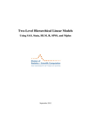
54Table 2. Sample dataset using the disaggregation method, with level-2 and level-3 variables excluded from the data(dataset is adapted from an example by Snijders & Bosker, 1999)Student ID(Level-1)12345678910Classroom ID(Level-2)1122334455School ID(Level-3)11111111111 variable breakfast consumption affects student GPA,disaggregation would entail studying level-2 and level-3variables at level-1. All students in the same class would beassigned the same mean classroom-related scores (e.g.,homework assignment load, teaching experience, andteaching style ratings), and all students in the same schoolwould be assigned the same mean school-related scores(e.g., school geographic location and annual budget ratings;see Table 2).By bringing upper level variables down to level-1,shared variance is no longer accounted for and theassumption of independence of errors is violated. If teachingstyle influences student breakfast consumption, for example,the effects of the level-1 (student) and level-2 (classroom)variables on the outcome of interest (GPA) cannot bedisentangled. In other words, the impact of being taught inthe same classroom on students is no longer accounted forwhen partitioning variance using the disaggregationapproach. Dependencies in the data remain uncorrected, theassumption of independence of observations required forsimple regression is violated, statistical tests are based onlyon the level-1 sample size, and the risk of partitioningvariance incorrectly and making inaccurate statisticalestimates increases (Beaubien et al., 2001; Gill, 2003;Osborne, 2000). As a general rule, HLM is recommendedover disaggregation for dealing with nested data because itaddresses each of these statistical limitations.In Figure 1, depicting the relationship between breakfastconsumption and student GPA using disaggregation, thepredictor variable (breakfast consumption) is negativelyrelated to the outcome variable (GPA). Despite (X, Y) unitsbeing situated variably above and below the regression line,this method of analysis indicates that, on average, unitincreases in a student’s breakfast consumption result in alowering of that student’s GPA.GPA Score(Level-1)5746352413Breakfast Consumption Score(Level-1)1324354657AggregationAggregation of data deals with the issues of hierarchicaldata analysis differently than disaggregation: Instead ofignoring higher level group differences, aggregation ignoreslower level individual differences. Level-1 variables areraised to higher hierarchical levels (e.g., level-2 or level-3)and information about individual variability is lost. Inaggregated statistical models, within-group variation isignored and individuals are treated as homogenous entities(Beaubien et al., 2001; Gill, 2003; Osborne, 2000). To theresearcher investigating the impact of breakfastconsumption on student GPA, this approach changes theresearch question (Osborne, 2000). Mean classroom GPAbecomes the new outcome variable of interest, rather thanFigure 1. The relationship between breakfast consumptionand student GPA using the disaggregation method. Figureis adapted from an example by Snijders & Bosker (1999) andStevens (2007).
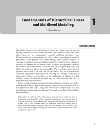
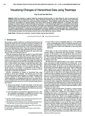
55Table 3. Sample dataset using the aggregation method, with level-1 variables excluded from the data(dataset is adapted from an example by Snijders & Bosker, 1999)Teacher ID(Level-2)12345Classroom GPA(Level-2)65432student GPA. Also, variation in students’ breakfast habits isno longer measurable; instead, the researcher must usemean classroom breakfast consumption as the predictorvariable (see Table 3 and Figure 2). Up to 80-90% ofvariability due to individual differences may be lost usingaggregation, resulting in dramatic misrepresentations of therelationships between variables (Raudenbush & Bryk, 1992).HLM is generally recommended over aggregation fordealing with nested data because it effectively disentanglesindividual and group effects on the outcome variable.In Figure 2, depicting the relationship betweenclassroom breakfast consumption and classroom GPA usingaggregation, the predictor variable (breakfast consumption)is again negatively related to the outcome variable (GPA). Inthis method of analysis, all (X, Y) units are situated on theregression line, indicating that unit increases in aclassroom’s mean breakfast consumption perfectly predict alowering of that classroom’s mean GPA. Although anegative relationship between breakfast consumption andGPA is found using both disaggregation and aggregationtechniques, breakfast consumption is found to impact GPAmore unfavourably using aggregation.Figure 2. The relationship between classroom breakfastconsumption and classroom GPA using the aggregationmethod. Figure is adapted from an example by Snijders &Bosker (1999) and Stevens (2007).Classroom Breakfast Consumption(Level-2)23456HLMFigure 3 depicts the relationship between breakfastconsumption and student GPA using HLM. Each level-1(X,Y) unit (i.e., each student’s GPA and breakfastconsumption) is identified by its level-2 cluster (i.e., thatstudent’s classroom). Each level-2 cluster’s slope (i.e., eachclassroom’s slope) is also identified and analyzed separately.Using HLM, both the within- and between-groupregressions are taken into account to depict the relationshipbetween breakfast consumption and GPA. The resultinganalysis indicates that breakfast consumption is positivelyrelated to GPA at level-1 (i.e., at the student level) but thatthe intercepts for these slope effects are influenced by level-2factors [i.e., students’ breakfast consumption and GPA (X, Y)units are also affected by classroom level factors]. Althoughdisaggregation and aggregation methods indicated anegative relationship between breakfast consumption andGPA, HLM indicates that unit increases in breakfastconsumption actually positively impact GPA. Asdemonstrated, HLM takes into consideration the impact ofFigure 3. The relationship between breakfast consumptionand student GPA using HLM. Figure is adapted from anexample by Snijders & Bosker (1999) and Stevens (2007).
56factors at their respective levels on an outcome of interest. Itis the favored technique for analyzing hierarchical databecause it shares the advantages of disaggregation andaggregation without introducing the same disadvantages.As highlighted in this example, HLM can be ideallysuited for the analysis of nested data because it identifies therelationship between predictor and outcome variables, bytaking both level-1 and level-2 regression relationships intoaccount. Readers who are interested in exploring thedifferences yielded by aggregation and disaggregationmethods of analysis compared to HLM are invited toexperiment with the datasets provided. Level-1 and level-2datasets are provided to allow readers to follow along withthe HLM tutorial in section 4 and to practice running anHLM. An aggregated version of these datasets is alsoprovided for readers who would like to compare the resultsyielded from an HLM to those yielded from a regression.In addition to HLM’s ability to assess cross-level datarelationships and accurately disentangle the effects ofbetween- and within-group variance, it is also a preferredmethod for nested data because it requires fewerassumptions to be met than other statistical methods(Raudenbush & Bryk, 2002). HLM can accommodate nonindependence of observations, a lack of sphericity, missingdata, small and/or discrepant group sample sizes, andheterogeneity of variance across repeated measures. Effectsize estimates and standard errors remain undistorted andthe potentially meaningful variance overlooked usingdisaggregation or aggregation is retained (Beaubien,Hamman, Holt & Boehm-Davis, 2001; Gill, 2003; Osborne,2000).A disadvantage of HLM is that it requires large samplesizes for adequate power. This is especially true whendetecting effects at level-1. However, higher-level effects aremore sensitive to increases in groups than to increases inobservations per group. As well, HLM can only handlemissing data at level-1 and removes groups with missingdata if they are at level-2 or above. For both of these reasons,it is advantageous to increase the number of groups asopposed to the number of observations per group. A studywith thirty groups with thirty observations each (n 900)can have the same power as one hundred and fifty groupswith five observations each (n 750; Hoffman, 1997).Equations Underlying Hierarchical Linear ModelsWe will limit our remaining discussion to two-levelhierarchical data structures concerning continuous outcome(dependent) variables as this provides the most thorough,yet simple, demonstration of the statistical features of HLM.We will be using the notation employed by Raudenbush andBryk (2002; see Raudenbush & Bryk, 2002 for three-levelmodels; see Wong & Mason, 1985 for dichotomous outcomevariables). As stated previously, hierarchical linear modelsallow for the simultaneous investigation of the relationshipwithin a given hierarchical level, as well as the relationshipacross levels. Two models are developed in order to achievethis: one that reflects the relationship within lower levelunits, and a second that models how the relationship withinlower level units varies between units (thereby correctingfor the violations of aggregating or disaggregating data;Hofmann, 1997). This modeling technique can be applied toany situation where there are lower-level units (e.g., thestudent-level variables) nested within higher-level units(e.g., classroom level variables).To aid understanding, it helps to conceptualize thelower-level units as individuals and the higher-level units asgroups. In two-level hierarchical models, separate level-1models (e.g., students) are developed for each level-2 unit(e.g., classrooms). These models are also called within-unitmodels as they describe the effects in the context of a singlegroup (Gill, 2003). They take the form of simple regressionsdeveloped for each individual i:(1)where: dependent variable measured for ith level-1 unitnested within the jth level-2 unit, value on the level-1 predictor, intercept for the jth level-2 unit, regression coefficient associated withfor the jthlevel-2 unit, and random error associated with the ith level-1 unitnested within the jth level-2 unit.In the context of our example, these variables can beredefined as follows: GPA measured for student i in classroom j breakfast consumption for student i in classroom j GPA for student i in classroom j who does not eatbreakfast regression coefficient associated with breakfastconsumption for the jth classroom random error associated with student i in classroomj.As with most statistical models, an importantassumption of HLM is that any level-1 errors ( ) follow anormal distribution with a mean of 0 and a variance of(see Equation 2; Sullivan, Dukes & Losina, 1999). Thisapplies to any level-1 model using continuous outcomevariables.(2)
57In the level-2 models, the level-1 regression coefficientsand) are used as outcome variables and are related(to each of the level-2 predictors. Level-2 models are alsoreferred to as between-unit models as they describe thevariability across multiple groups (Gill, 2003). We willconsider the case of a single level-2 predictor that will bemodeled using Equations 3 and 4:(3)(4)where: intercept for the jth level-2 unit; slope for the jth level-2 unit; value on the level-2 predictor; overall mean intercept adjusted for G; overall mean intercept adjusted for G; regression coefficient associated with G relative tolevel-1 intercept; regression coefficient associated with G relative tolevel-1 slope; random effects of the jth level-2 unit adjusted for Gon the
Hierarchical Linear Modeling (HLM) is a complex form of ordinary least squares (OLS) regression that is used to analyze variance in the outcome variables when the predictor variables are at varying hierarchical levels; for example, students in a classroom share variance ac