WIXLIB

Chapter 5Log-Linear Models forContingency TablesIn this chapter we study the application of Poisson regression models tothe analysis of contingency tables. This is perhaps one of the most popularapplications of log-linear models, and is based on the existence of a veryclose relationship between the multinomial and Poisson distributions.5.1Models for Two-dimensional TablesWe start by considering the simplest possible contingency table: a two-bytwo table. However, the concepts to be introduced apply equally well tomore general two-way tables where we study the joint distribution of twocategorical variables.5.1.1The Heart Disease DataTable 5.1 was taken from the Framingham longitudinal study of coronaryheart disease (Cornfield, 1962; see also Fienberg, 1977). It shows 1329 patients cross-classified by the level or their serum cholesterol (below or above260) and the presence or absence of heart disease.There are various sampling schemes that could have led to these data,with consequences for the probability model one would use, the types ofquestions one would ask, and the analytic techniques that would be employed. Yet, all schemes lead to equivalent analyses. We now explore severalapproaches to the analysis of these data.G. Rodrı́guez. Revised November, 2001; minor corrections August 2010, February 2014

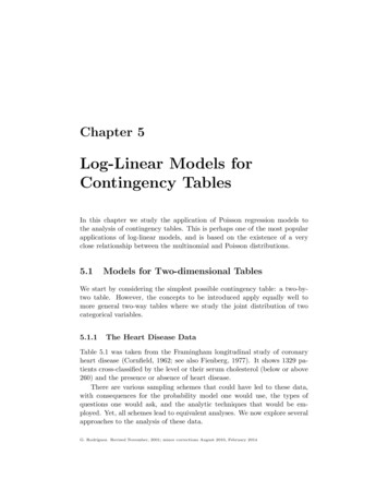
2CHAPTER 5. LOG-LINEAR MODELSTable 5.1: Serum Cholesterol and Heart DiseaseSerumCholesterol 260260 Total5.1.2Heart DiseasePresent Absent5199241245921237Total10432861329The Multinomial ModelOur first approach will assume that the data were collected by sampling 1329patients who were then classified according to cholesterol and heart disease.We view these variables as two responses, and we are interested in their jointdistribution. In this approach the total sample size is assumed fixed, and allother quantities are considered random.We will develop the random structure of the data in terms of the row andcolumn variables, and then note what this implies for the counts themselves.Let C denote serum cholesterol and D denote heart disease, both discretefactors with two levels. More generally, we can imagine a row factor with Ilevels indexed by i and a column factor with J levels indexed by j, formingan I J table. In our example I J 2.To describe the joint distribution of these two variables we let πij denotethe probability that an observation falls in row i and column j of the table.In our example words, πij is the probability that serum cholesterol C takesthe value i and heart disease D takes the value j. In symbols,πij Pr{C i, D j},(5.1)for i 1, 2, . . . , I and j 1, 2, . . . , J. These probabilities completely describethe joint distribution of the two variables.We can also consider the marginal distribution of each variable. Let πi.denote the probability that the row variable takes the value i, and let π.jdenote the probability that the column variable takes the value j. In ourexample πi. and π.j represent the marginal distributions of serum cholesteroland heart disease. In symbols,πi. Pr{C i}andπ.j Pr{D j}.(5.2)Note that we use a dot as a placeholder for the omitted subscript.The main hypothesis of interest with two responses is whether they areindependent. By definition, two variables are independent if (and only if)

5.1. MODELS FOR TWO-DIMENSIONAL TABLES3their joint distribution is the product of the marginals. Thus, we can writethe hypothesis of independence asH0 : πij πi. π.j(5.3)for all i 1, . . . , I and j 1, . . . , J. The question now is how to estimatethe parameters and how to test the hypothesis of independence.The traditional approach to testing this hypothesis calculates expectedcounts under independence and compares observed and expected counts using Pearson’s chi-squared statistic. We adopt a more formal approach thatrelies on maximum likelihood estimation and likelihood ratio tests. In orderto implement this approach we consider the distribution of the counts in thetable.Suppose each of n observations is classified independently in one of theIJ cells in the table, and suppose the probability that an observation fallsin the (i, j)-th cell is πij . Let Yij denote a random variable representingthe number of observations in row i and column j of the table, and let yijdenote its observed value. The joint distribution of the counts is then themultinomial distribution, withPr{Y y} n!π y11 π y12 π y21 π y22 ,y11 !y12 !y21 !y22 ! 11 12 21 22(5.4)where Y is a random vector collecting all four counts and y is a vectorof observed values. The term to the right of the fraction represents theprobability of obtaining y11 observations in cell (1,1), y12 in cell (1,2), andso on. The fraction itself is a combinatorial term representing the numberof ways of obtaining y11 observations in cell (1,1), y12 in cell (1,2), and soon, out of a total of n. The multinomial distribution is a direct extensionof the binomial distribution to more than two response categories. In thepresent case we have four categories, which happen to represent a two-bytwo structure. In the special case of only two categories the multinomialdistribution reduces to the familiar binomial.Taking logs and ignoring the combinatorial term, which does not dependon the parameters, we obtain the multinomial log-likelihood function, whichfor a general I J table has the formlog L I XJXyij log(πij ).(5.5)i 1 j 1To estimate the parameters we need to take derivatives of the log-likelihoodfunction with respect to the probabilities, but in doing so we must take into

4CHAPTER 5. LOG-LINEAR MODELSaccount the fact that the probabilities add up to one over the entire table.This restriction may be imposed by adding a Lagrange multiplier, or moresimply by writing the last probability as the complement of all others. Ineither case, we find the unrestricted maximum likelihood estimate to be thesample proportion:yijπ̂ij .nSubstituting these estimates into the log-likelihood function gives its unrestricted maximum.Under the hypothesis of independence in Equation 5.3, the joint probabilities depend on the margins. Taking derivatives with respect to πi. andπ.j , and noting that these are also constrained to add up to one over therows and columns, respectively, we find the m.l.e.’sπ̂i. yi.nandπ̂.j y.j,nPwhere yi. j yij denotes the row totals and y.j denotes the column totals.Combining these estimates and multiplying by n to obtain expected countsgivesyi. y.jµ̂ij ,nwhich is the familiar result from introductory statistics. In our example, theexpected frequencies areµ̂ij 72.2 970.819.8 266.2!.Substituting these estimates into the log-likelihood function gives its maximum under the restrictions implied by the hypothesis of independence. Totest this hypothesis, we calculate twice the difference between the unrestricted and restricted maxima of the log-likelihood function, to obtain thedeviance or likelihood ratio test statisticXXyij(5.6)D 2yij log( ).µ̂ijijNote that the numerator and denominator inside the log can be written interms of estimated probabilities or counts, because the sample size n cancelsout. Under the hypothesis of independence, this statistic has approximatelyin large samples a chi-squared distribution with (I 1)(J 1) d.f.Going through these calculations for our example we obtain a devianceof 26.43 with one d.f. Comparison of observed and fitted counts in terms of

5.1. MODELS FOR TWO-DIMENSIONAL TABLES5Pearson’s chi-squared statistic gives 31.08 with one d.f. Clearly, we rejectthe hypothesis of independence, concluding that heart disease and serumcholesterol level are associated.5.1.3The Poisson ModelAn alternative model for the data in Table 5.1 is to treat the four counts asrealizations of independent Poisson random variables. A possible physicalmodel is to imagine that there are four groups of people, one for each cell inthe table, and that members from each group arrive randomly at a hospitalor medical center over a period of time, say for a health check. In this modelthe total sample size is not fixed in advance, and all counts are thereforerandom.Under the assumption that the observations are independent, the jointdistribution of the four counts is a product of Poisson distributionsyPr{Y y} Y Y µijij e µijijyij !.(5.7)Taking logs we obtain the usual Poisson log-likelihood from Chapter 4.In terms of the systematic structure of the model, we could consider threelog-linear models for the expected counts: the null model, the additive modeland the saturated model. The null model would assume that all four kindsof patients arrive at the hospital or health center in the same numbers. Theadditive model would postulate that the arrival rates depend on the levelof cholesterol and the presence or absence of heart disease, but not on thecombination of the two. The saturated model would say that each group hasits own rate or expected number of arrivals.At this point you may try fitting the Poisson additive model to the fourcounts in Table 5.1, treating cholesterol and heart disease as factors or discrete predictors. You will discover that the deviance is 26.43 on one d.f. (fourobservations minus three parameters, the constant and the coefficients of twodummies representing cholesterol and heart disease). If you print the fittedvalues you will discover that they are exactly the same as in the previoussubsection.This result, of course, is not a coincidence. Testing the hypothesis ofindependence in the multinomial model is exactly equivalent to testing thegoodness of fit of the Poisson additive model. A rigorous proof of this resultis beyond the scope of these notes, but we can provide enough informationto show that the result is intuitively reasonable and to understand when itcan be used.