Transcription
Introduction to vector and tensor analysisJesper Ferkinghoff-BorgSeptember 6, 2007
Contents1 Physical space1.1 Coordinate systems . . . . . . . . . . . . . . . . . . . . . . . . . .1.2 Distances . . . . . . . . . . . . . . . . . . . . . . . . . . . . . . .1.3 Symmetries . . . . . . . . . . . . . . . . . . . . . . . . . . . . . .2 Scalars and vectors2.1 Definitions . . . . . . . . . . . . . . . . . . . .2.2 Basic vector algebra . . . . . . . . . . . . . .2.2.1 Scalar product . . . . . . . . . . . . .2.2.2 Cross product . . . . . . . . . . . . . .2.3 Coordinate systems and bases . . . . . . . . .2.3.1 Components and notation . . . . . . .2.3.2 Triplet algebra . . . . . . . . . . . . .2.4 Orthonormal bases . . . . . . . . . . . . . . .2.4.1 Scalar product . . . . . . . . . . . . .2.4.2 Cross product . . . . . . . . . . . . . .2.5 Ordinary derivatives and integrals of vectors .2.5.1 Derivatives . . . . . . . . . . . . . . .2.5.2 Integrals . . . . . . . . . . . . . . . . .2.6 Fields . . . . . . . . . . . . . . . . . . . . . .2.6.1 Definition . . . . . . . . . . . . . . . .2.6.2 Partial derivatives . . . . . . . . . . .2.6.3 Differentials . . . . . . . . . . . . . . .2.6.4 Gradient, divergence and curl . . . . .2.6.5 Line, surface and volume integrals . .2.6.6 Integral theorems . . . . . . . . . . . .2.7 Curvilinear coordinates . . . . . . . . . . . .2.7.1 Cylindrical coordinates . . . . . . . .2.7.2 Spherical coordinates . . . . . . . . . .3334555677910111112131414151515161720242627283 Tensors303.1 Definition . . . . . . . . . . . . . . . . . . . . . . . . . . . . . . . 303.2 Outer product . . . . . . . . . . . . . . . . . . . . . . . . . . . . 313.3 Basic tensor algebra . . . . . . . . . . . . . . . . . . . . . . . . . 311
.3233333435383839404 Tensor calculus4.1 Tensor notation and Einsteins summation rule .4.2 Orthonormal basis transformation . . . . . . . .4.2.1 Cartesian coordinate transformation . . .4.2.2 The orthogonal group . . . . . . . . . . .4.2.3 Algebraic invariance . . . . . . . . . . . .4.2.4 Active and passive transformation . . . .4.2.5 Summary on scalars, vectors and tensors .4.3 Tensors of any rank . . . . . . . . . . . . . . . .4.3.1 Introduction . . . . . . . . . . . . . . . .4.3.2 Definition . . . . . . . . . . . . . . . . . .4.3.3 Basic algebra . . . . . . . . . . . . . . . .4.3.4 Differentiation . . . . . . . . . . . . . . .4.4 Reflection and pseudotensors . . . . . . . . . . .4.4.1 Levi-Civita symbol . . . . . . . . . . . . .4.4.2 Manipulation of the Levi-Civita symbol .4.5 Tensor fields of any rank . . . . . . . . . . . . . .42434445454647484949505153545556573.43.53.3.1 Transposed tensors . . . . . . . . .3.3.2 Contraction . . . . . . . . . . . . .3.3.3 Special tensors . . . . . . . . . . .Tensor components in orthonormal bases .3.4.1 Matrix algebra . . . . . . . . . . .3.4.2 Two-point components . . . . . . .Tensor fields . . . . . . . . . . . . . . . . .3.5.1 Gradient, divergence and curl . . .3.5.2 Integral theorems . . . . . . . . . .5 Invariance and symmetries.602
Chapter 1Physical space1.1Coordinate systemsIn order to consider mechanical -or any other physical- phenomena it is necessary to choose a frame of reference, which is a set of rules for ascribing numbersto physical objects. The physical space has three dimensions, which means thatit takes exactly three numbers -say x1 , x2 , x3 - to locate a point, P , in space.These numbers are called coordinates of a point, and the reference frame for thecoordinates is called the coordinate system C. The coordinates of P can conveniently be collected into a a triplet, (x)C (P ) (x1 (P ), x2 (P ), x3 (P ))C , calledthe position of the point. Here, we use an underline simply as a short hand notation for a triplet of quantities. The same point will have a different position(x0 )C 0 (P ) (x01 (P ), x02 (P ), x03 (P ))C 0 in a different coordinate system C 0 . However, since difference coordinate systems are just different ways of representingthe same physical space in terms of real numbers, the coordinates of P in C 0must be a unique function of its coordinates in C. This functional relation canbe expressed asx0 x0 (x)(1.1)which is a shorthand notation forx01x02x03 x01 (x1 , x2 , x3 ) x02 (x1 , x2 , x3 ) x03 (x1 , x2 , x3 )(1.2)This functional relation is called a coordinate transformation. The inverse transformation must also exist, because both systems are assumed to cover the samespace.1.2Distances.3
We will take it for given that one can ascribe a unique value (ie. independent of the chosen coordinate system), D(O, P ), for the distance between twoarbitraily chosen points O and P . Also we assume (or we may take it as anobservational fact) that when D becomes sufficiently small, a coordinate systemexists by which D can be calculated according to Pythagoras law:vu duXD(O, P ) t (xi (P ) xi (O))2 , Cartesian coordinate system,(1.3)i 1where d 3 is the dimension.We will call such a coordinate system a Cartesian or a Rectangular coordinatesystem. Without loss of generality we can choose one of the points as origen,-say O-, so x(O) (0, 0, 0). The neighborhood, Ω(O), around O for whichdistances between any two points, P1 , P2 Ω(O) can be calculated accordingto Eq. (1.3) for the same fixed coordinate system is coined a (local) Euklideanspace. In an Euklidean space, we also write P1 P2 for D(P1 , P2 ), representingthe length of the line segment connecting P1 and P2 . Trivially, O Ω(O).Classical physics takes place in a 3-dimensional globally Euclidean spaceΩ(O) R3 . In general relativity space are intrinsically curved and the assumption of an Euklidean space can only be applied locally. The principle ofcurved space is easier to envisage for 2d-surfaces. For instance all points on thesurface of earth can be represented by two numbers -say x1 , x2 - representingthe longitude and latitude. However, the law of Pythagoras (with d 2) canonly be applied for small rectangular triangles1 on the surface, ie. locally. Forlarger rectangular triangles the sum of the angles will be larger than 1800 andPythagoras’ law will not be correct. All geometric analysis, however, rely onthe assumption that at sufficently small scales the space will appear flat. Indifferential geometry one only requires flatness in a differential sence.1.3SymmetriesFor classical mechanical phenomena it is found that a frame of reference canalways be chosen in which space is homogeneous and isotropic and time is homogeneous. It implies that nature has no sence of an absolute origin in timeand space and no sence of an absolute direction. Mechanical or geometrical lawsshould therefore be invariant to coordinate transformations involving rotationsand translations. Motivated by this fact we are inclined to develop a mathematical formalism for operating with geometrical objects without referring to acoordinate system or, equivalently, a formalism which will take the same form(ie. is covariant) for all coordinates. This fundamental principle is called theprinciple of covariance. The mathematics of scalar, vector and tensor algebra isprecisely such a formalism.1 Small would mean that the length of line segments are much smaller than the radius ofearth4
Chapter 2Scalars and vectors2.1DefinitionsA vector is a quantity having both magnitude and a direction in space, such asdisplacement, velocity, force and acceleration.Graphically a vector is represented by an arrow OP from a point O to apoint P , defining the direction and the magnitude of the vector being indicatedby the length of the arrow. Here, O is called the initial point and P is called the or OP andterminal point. Analytically, the vector is represented by either OP the magnitude by OP or OP . We shall use the bold face notation in thesenotes. In this chapter will assume that all points P belong to an Euklideanspace, P Ω(O), meaning that lengths of line segments can be calculatedaccording to Pythagoras.A scalar is a quantity having magnitude but no direction, e.g. mass, length,time, temperature and any real number.We indicate scalars by letters of ordinary types. For example, a vector a willhave length a a . Operations with scalars follow the same rules as elementaryalgebra; so multiplication, addition and substraction (provided the scalars havesame units) follow the usual algebraic rules.2.2Basic vector algebraThe operations defined for real numbers are, with suitable definitions, capableof extension to an algebra of vectors. The following definitions are fundamentaland define the basic algebraic rules of vectors:1. Two vectors a and b are equal if they have the same magnitude anddirection regardless of the position of their initial point.2. A vector having direction opposite of a vector a but having the samemagnitude is denoted a.5
3. The sum of resultant of vectors a and b is a vector c formed by placingthe initial point of b on the terminal point of a and then joining the initialpoint of a to the terminal point of b. The sum is written c a b.4. The difference between two vectors, a and b, represented by a b isdefined as the sum a ( b).5. The product of a vector a with a scalar m is a vector ma with magnitude m times the magnitude of a, ie ma m a , and with direction thesame as or opposite to that of a, according as m is positive or negative.We stress that these definitions for vector addition, substraction and scalarmultiplications are defined geometrically, ie. they have no reference to coordinates. It then becomes a pure geometric exercise to prove the following laws:a ba (b c)m(na)(m n)am(a b)am b a (a b) c (mn)a ma na ma nb def amCommutative law for additionAssociate law for additionAssociate law for multiplicationDistributive lawDistributive lawCommutative law for multiplication(2.1)Here, the last formula should just be read as a definition of a vector times ascalar. Note that in all cases only multiplication of a vector by one or morescalars are defined. One can define different types of bilinear vector products.The three basic types are called scalar product (or inner product), cross productand outer product (or tensor product). We shall define each in turn. Thedefinition of the outer product is postponed to chapter 3.Following definition will become useful:A unit vector is a vector having unit magnitude. If a is not a null vectorthen a/ a is a unit vector having the same direction as a.2.2.1Scalar productThe scalar product between two vectors, a and b is defined bya · b ab cos(θ),0 θ π(2.2)where a a , b b and θ is the angle between the two vectors. Note thata · b is a scalar. Following rules apply:a·b(a b) · ca · (b c)m(a · b) b·a a·c b·c a·b a·c (ma) · b a · (mb)Commutative law for scalar productDistributive law in 1. argumentDistributive law for 2. argmentm is a scalar(2.3)6
The three last formulas make the scalar product bilinear in the two arguments.Note also,1 a · a a 22 If a · b 0 and a and b are not null vectors,then a and b are perpendicular.3 The projection of a vector a on b is equal to a · eb ,where eb b/ b is the unit vector in direction of b.2.2.2(2.4)Cross productThe cross product, a b between two vectors a and b is a vector defined bya b ab sin(θ)u, 0 θ π,(2.5)where θ is the angle between a and b and u is a unit vector in the directionperpendicular to the plane of a and b such that a, b and u form a right-handedsystem1 .The following laws are valid:a b(a b) ca (b c)m(a b) b a a c b c a b a c (ma) b a (mb)Cross product is not commutative.Distributive law for 1. argumentDistributive law for 2. argumentm is a scalar(2.6)The last three formulas make the cross product bilinear.Note that:1. The absolute value of the cross product a b has a particular geometricmeaning. It equals the area of the parallelogram spanned by a and b.2. The absolute value of the triple product a·(b c) has a particular geometricmeaning. It equals the volume of the parallelepiped spanned by a, b andc2.3Coordinate systems and basesWe emphasize again that all definitions and laws of vector algebra, as introducedabove, are invariant to the choise of coordinate system2 . Once we introduce away of ascribing positions to points by the choise of a coordinate system, C, weobtain a way of representing vectors in terms of triplets.1 It is seen that the definition of the cross-product explicitly depends on an arbitrary choiseof handedness. A vector whose direction depends on the choise of handedness is called anaxial vector or pseudovector as opposed to ordinary or polar vectors, whose directions areindependent of the choise of handedness.2 With the one important exception that we have assumed the absolute notion of handednessin the definition of the cross product.7
By assumption, we can choose this coordinate system to be rectangular(R), CR , cf. chapter 1. By selecting four points O, P1 , P2 and P3 having thecoordinatesxCR (O) (0, 0, 0), xCR (P1 ) (1, 0, 0), xCR (P2 ) (0, 1, 0), xCR (P3 ) (0, 0, 1)(2.7)we can construct three vectorse1 OP1 , e2 OP2 , e3 OP3 .(2.8)Furthermore, from the choise of an origin O, a position vector, r OP, can beassociated to any point P by the formulaXxi (P )eiCR rectangular.(2.9)r(P ) r(xCR (P )) iThe position vector is an improper vector, meaning that it explicitly depends onthe position of its initial point O. It will therefore change upon a transformationt
2.2.2 Cross product The cross product, a b between two vectors a and b is a vector de ned by a b absin( )u; 0 ˇ; (2.5) where is the angle between a and b and u is a unit vector in the direction perpendicular to the plane of a and b such that a;b and u form