Transcription
Finite Element Method for 1D TransientConvective Heat Transfer ProblemsWhokko SchirénJune 24, 2018
iiAcknowledgementI would like to express my deep gratitude to Björn Johannesson andKarl-Olof Lindahl, my supervisors in this thesis work. Without theirvaluable support and advice, their unwavering encouragement and trustand their valuable critique, this work would not have been possible. I alsowant to thank Winston Mmari who has been of great help in bringing thiswork forth and Marko Sobak who’s comments improved the quality of thework.Finally I would like to thank my family for their great patience andsupport.
iiiAbstractWe study heat transfer in one dimension with and without convection,also called advection-diffusion. This is done using the Finite ElementMethod (FEM) to discretise the mathematical model, i.e. the heat equation. The results are compared to analytic Fourier series solutions. Ourmain result is that the FEM could be used to better model the heat transfer which allow for more accurate models than today’s use of steady statemodels.Keywords: Advection-Diffusion; Convection; Convection Problems; Finite Element Method; FEM; Transient 1D Heat Equation; Discretisation
CONTENTSivContents1 Introduction12 Theory2.1 From strong formulation to weak . . . . . . . . . . . . . . . . . .2.1.1 1D heat equation without convection . . . . . . . . . . . .2.1.2 1D heat equation with convection . . . . . . . . . . . . .34453 Result and Analysis3.1 Finite element models . . . . . . . . . . . . . . . . . . . . . . . .3.1.1 Discretisation in space of the 1D heat equation withoutconvection . . . . . . . . . . . . . . . . . . . . . . . . . . .3.1.2 Discretisation in time of the 1D heat equation withoutconvection . . . . . . . . . . . . . . . . . . . . . . . . . . .3.1.3 Discretisation in space of the 1D heat equation with convection . . . . . . . . . . . . . . . . . . . . . . . . . . . .3.1.4 Discretisation in time of the 1D heat equation with convection . . . . . . . . . . . . . . . . . . . . . . . . . . . .3.2 Finite element implementation . . . . . . . . . . . . . . . . . . .3.3 Condition numbers . . . . . . . . . . . . . . . . . . . . . . . . . .3.4 Analytical solutions . . . . . . . . . . . . . . . . . . . . . . . . .3.4.1 Analytical solution of the 1D heat equation without convection . . . . . . . . . . . . . . . . . . . . . . . . . . . .3.4.2 Analytical solution for 1D heat transfer with convection .3.5 Comparison between FEM and analytical solutions . . . . . . . .774 Discussion710121617192222272831Appendix A FE-model & analytical, without convectionA-1Appendix B FE-model & analytical, with convectionB-1Appendix C Condition numbers, without convectionC-1Appendix D Condition numbers, with convectionD-1
11INTRODUCTION1IntroductionThis work focuses on the study of one dimensional transient heat transfer. Thisis of interest to the construction industry as heat and moisture levels are interdependent and moisture is a risk factor in buildings. If the relative humiditygets too high we might get moisture problems. The relative humidity dependson the temperature as air with higher temperature can hold more moisture,moisture that risks being turned into condensation if the temperature drops,and if we get condensation, let us say inside a wall, then we have got moistureproblems. Furthermore, we often have different air pressure inside and outsidea building and this difference could affect the temperature distribution insidethe wall as the difference in pressure pushes warm air through the wall, thisphenomenon is called convection, or, in some literature, advection-diffusion. Itis therefore of great interest to simulate the temperature distribution througha wall, with and without convection. We are especially interested in how thetemperature changes over time after a temperature change has been made onone side of the wall and before the steady state situation has been reached.Every model is an idealisation of the real world and, as George Box put it,”All models are wrong; some are useful” [3, p. 1–10]. We start out with a physicalsystem, heat transfer through a wall, this system we idealise as a mathematicalmodel which we then do a discretisation on using the finite element method,this gives us a discrete solution. As a mathematical model we use the heatequation with and without an added convection term. We discretise the modelusing the Finite Element Method (FEM), this gives us a discrete problem. Westart by deriving the steady state heat balance equation, then we find the strongand the weak formulation for the one dimensional heat equation, in space andtime. This will be done for two cases, with and without convection. In each ofthese steps there could arise errors as we do approximations and simplifications,see Figure 1. The discrete solution could give solution errors, there could beFigure 1: Simulation process, Figure 6.1 in [3].discretisation errors given how we have done the discretisation and there couldexist modelling errors depending on the choice of idealisation. Typically thesolution errors will be small compared to the modelling errors which arise when
1INTRODUCTION2we make a model of a physical system. The only way to check these errors isby comparison to a physical system. This has not been done in this work, weinstead start from a mathematical model to obtain analytical solutions whichwe can compare our discrete solutions against.A significant part of the work is how to handle the case with convection asthe standard numerical assumptions are not optimal when working with transport equations such as the convection equation for heat transfer. In FEM itis common to use the Galerkin method when choosing the weight function, i.e.the weight function is described by the shape function. In another numericalmethod, the finite difference method, the central difference scheme is typicallyused to approximate the state function in the spatial domain. None of thesemethods, the Galerkin method nor the central difference scheme, can correctlysolve the convection equation when the convection velocity is strong comparedto the conduction. In this work we will use the Petrov-Galerkin method asan approach to improve the solutions to the problem with convection. In thePetrov-Galerkin method the weight function is adjusted so that the analyticalsolution for a linear steady state problem is obtained. That is, the weight function is chosen so that the analytical and numerical steady state solutions matchexactly at the nodal points. For this purpose we define a so-called elementPéclet number as a function of the local elements spatial length, the conductionand the convection velocity. For high element Péclet numbers the convectionvelocity is large compared to the other properties included in its definition andthe effect of using a proper weighting becomes more and more important. Weinvestigate the convection equation together with its transient behaviour, thatis, the change of the temperature with time is considered together with theheat capacity. In this work we take a analytical solution of a one dimensionalconvection equation from the literature and compare it to a developed transientfinite element scheme. A part of the problem is that the time stepping scheme isderived for its unconditional stability using standard transport equations without convection. This means that for high element Péclet numbers the solutionsmay be polluted by oscillations for implicit stable schemes. In order to investigate the overall stability of the scheme different transient numerical simulationresults where produced and compared to the analytical solutions using implicittime integration.Next we implement our finite element models using MATLAB and check thecondition numbers for the cases with and without convection. We will also useMATLAB to calculate the heat transfer analytically and compare the results tothe results from the FEM implementations.We found that the FEM is stable and give insight into how temperaturechange over time in one dimension. We also learned that we have to be carefulabout how we choose the integration interval in time for the analytic solutionsas the solution otherwise could get too large solutions errors as it is based on aFourier series and there arise problems due to the truncation of the series.Now, as promised, we start our journey by deriving the heat equation.
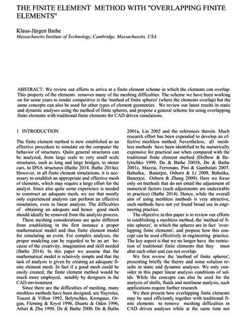
22THEORY3TheoryDerivation of the heat equationThe heat equation for steady state conditions, that is when there is no timedependency, could be derived by looking at an infinitely small part dx of a onedimensional heat conducting body which is heated by a stationary inner heatsource Q. By one dimensional we mean that the body is laterally insulated sothat heat can only flow along the element in the x-direction. We also assumethat the body is thin enough for the temperature to be constant within anygiven cross-section of the body.According to the law of energy conservation the amount of heat energy Hentering the body must be equal to the amount leaving it, as illustrated inFigure 2, soH Q dx H dH,ordH Q.dx(1)A definition of heat isH(x) A(x)q(x),where A is the cross-sectional area of the element and q denotes the heat flux,therefore we rewrite (1) asd(Aq) Q,dxthis is the conservation equation.Figure 2: Heat balance.Let u (x) be the temperature, k the heat conductivity and u/ x the changerate of the temperature with respect to the position, then the heat flux is givenby Fourier’s law of heat conduction asq k u. x(2)
2THEORY4To allow for the heat to change with the time t we add a term which takesinto account the time dependency. Let ρ be the density and c the heat capacityor the amount of energy needed to raise the temperature inside the element byone degree. Then u ρc (Aq) Q.(3) t xWe now substitute (2) into (3) to obtain the heat equation as u uρc Ak Q 0. t x xWe will use this one dimensional heat equation to formulate the strong versionof the problem. We will then reformulate this differential equation with itsboundary conditions in its weak form. This is the form that we will use in thefinite element (FE) approach.2.1From strong formulation to weakIn this section we do as in [8] and go from a so called strong form, consistingof a differential equation with boundary conditions, to a weak form needed forthe FE approach.2.1.11D heat equation without convectionStrong formIn our specific problem there is no internal heat source, therefore Q 0 whichresults in the following strong form of the one-dimensional heat flow u u Ak,(0 x L, t 0) ,(4)ρc t x xwith boundary conditionsu (0, t) a,u (L, t) b.As an initial condition we will useu (x, 0) 0.The boundary conditions a and b are considered known constants. Next wesearch for the weak formulation of the strong form.Weak formWe want to lower the degree of the right hand side of (4). This is achievedby multiplying the strong form with a weight function and integrating over theproblem domain, then by the use of Green-Gauss theorem we can separate theright hand side into two parts.
2THEORY5We start by multiplying the differential equation (4) by two weight functionsv(x) and w (t), one for the spatial domain and one for the time domain, and thenintegrate over each domain. This gives the following integrals, Z LZ L u uv(x)ρcv(x)dx Akdx(5) t x x00andZ tZw (t)0Lv(x)ρc0 udx dt tZ tLZw (t)0v(x)0 x Ak u x dx dt.We will use the first integral here, the second one will be used later in thediscretisation in time. Integrate the right hand side of (5) using integration byparts to get L Z L Z L v u u u v(x)Akdx v(x)AkAkdx.(6) x x x 0 x0 x0In two or three dimension problems we would instead use the Green–Gausstheorem. Next substitute for (6) in (5) and rearrange the result to obtain LZ LZ L v u u udx .(7)v(x)ρcAkdx v(x)Ak t x x 00 x0 Remembering that q denotes the flux allows for replacing k u x by q to get Z LZ L u u vLv(x)ρcdx Akdx [v(x)Aq]0 . t x x00This equation together with the same boundary conditions as before,u (0, t) a,u (L, t) b,make up the weak formulation of the one-dimensional heat equation. This weakformulation will be the basis for our finite element formulation of the problem,found in Section 3.1.1.2.1.21D heat equation with convectionStrong formulationWe know from the previous Section that u uρc Ak, t x xwhere the left hand side is the transient part and the right hand is a diffusionterm. In this section we put A 1 and add convection to the equation asdescribed in [10, pp. 13–15], u u uν̄ ρc k,(0 x L, t 0) ,(8) x t x x
2THEORY6the first term describes the transport of the quantity u by convection in a fieldof velocity ν̄. Equation (8) together with boundary conditionsu (0, t) a,u (L, t) b,make up the strong formulation of our problem.Weak formulationAs before we leave everything connected to time until the discretisation in time,Section 3.1.4, instead now we multiply by the weighting function v(x) and integrate, Z LZ LZ L u u uv(x) ν̄ dx v(x)ρcdx v(x)kdx.(9) x t x x000We then use integration by parts on the right hand side to getZ0L v(x) x uk x L Z L u u vdx v(x)k kdx x 0 x0 xwhich we put back into equation (9) and rearrange the terms to get our weakformulation as LZ LZ LZ L u u u u vv(x) ν̄ dx dx kdx v(x)k.v(x)ρc x t x x 0000 x Remembering that q k u x let us rewrite this asZ0L uv(x) ν̄ dx xZ0L udx v(x)ρc tZ0L v x uk x Ldx [v(x)Aq]0 . (10)This weak formulation, together with the same initial condition and boundaryconditions as in Section 2.1.1, will be used in our finite element formulation ofthe one-dimensional heat equation with convection found in Section 3.1.3.
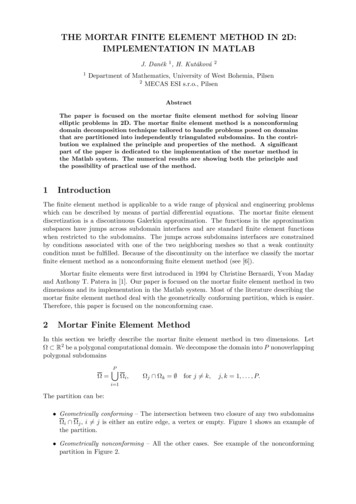
3RESULT AND ANALYSIS33.17Result and AnalysisFinite element modelsWe will now find the finite element formulations for one-dimensional heat flowwith and without convection, we use the method presented in [8].In the Finite Element Method, complex systems described by general differential equations can be solved approximately by dividing the system into anumber of small elements where the state for each element can be fairly simplycalculated. By this we mean that even if a variable varies non-linearly over theglobal system it could be an acceptable approximation to say that it varies linearly over each local element, if the size of the elements is small enough. Whenwe have decided the behaviour for all of these small elements they could be puttogether into a larger system approximately describing the whole system.3.1.1Discretisation in space of the 1D heat equation without convectionIn our case we deal with one dimensional heat transfer and so we divide ourglobal system of length L into a number of local elements of equal length h asin Figure 3. The points i, j, k and l are called nodes. To decide the tempera-Figure 3: Global system divided into local elements.ture over each of these elements we interpolate between the nodes using shapefunctions, later in this section we will get back to how the shape functions aredefined. Let the approximation of the temperature in an element be equal tou (x, t) Na.Both N and a are vectors,N NiNj ,a uiuj ,N denotes the shape functions and a the nodal temperatures of an element.The derivative of the temperatures with respect to the position, that is thetemperature gradient, is u (Na) Ba, x x
3RESULT AND ANALYSIS8where B x N and a is independent of x. If the derivative instead is takenwith respect to time, noting that N is independent of time, then the expressionbecome u a (Na) N Nȧ. t t tThe weight function v(x) is a scalar, therefore v must be equal to vT and theweight function can be approximated asv (x) Nc cT NT vT ,where N still denotes the shape functions and c is an arbitrary non-zero vector.This choice of weight function is in accordance with the Galerkin method wherethe test functions are put equal to the shape functions. For more information onweight functions and why the Galerkin method is a good choice see [8, pp. 142–156]. The derivative of the weight function is NT v cT cT BT . x xEach shape function has the property that it is equal to one at the node itcontrols and equal to zero in all other nodes, see Figure 4. In this case everythingis one dimensional and we choose linear shape functions, if an element has lengthh and goes from node 1 to 2 thenxN1e 1 ,(0 x h),hxN2e ,(0 x h),hthe superscript e denotes that these shape functions are for a local element. Theshape function vector for the studied case ishx xiN 1 ,h hwhich results in 1 1.B h hThe temperature vector is u1a ,u2where u1 and u2 are temperatures at the nodes 1 and 2. u vSubstituting for u, u x , t , v, and x in (7) gives the following equationZ hZ h hcT NT ρcNȧ dx cT BT AkBa dx cT NT Aq 0 .00TNext, we eliminate c , this is allowed as cT is an arbitrary non-zero vector. Weare left withZ hZ h hTN ρcNȧ dx BT AkBa dx NT Aq 000
3RESULT AND ANALYSIS9Figure 4: Linear element shape functions.which could be written in a compact form asCȧ Ka f(11)withZhNT ρcN dx,C 0ZK hBT AkB dx,0 hf NT Aq 0 ,where C is called the damping matrix, K the stiffness matrix, or more accuratelythe conductivity matrix, and f the force vector. Note that if the force vector issimplified we end up with 1f Aq. 1In this section we set up the system of linear equations for an element but(11) is easily expanded to apply to a global system of linear equations. Asan example let us take the stiffness matrix K and expand it to fit the systemshown in Figure 3. We ignore all constants for the sake of the argument, thenthe stiffness of a local element is 1 1Ke , 1 1where the superscript e clarifies that this is indeed the stiffness of a local element.Then for the global system we assemble the local stiffness matrices based onour knowledge about the elements location in the global system. We know thatelement one go from node i to j, element two go from node j to k, and so on.
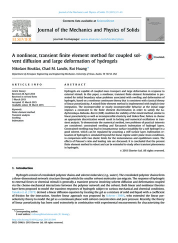
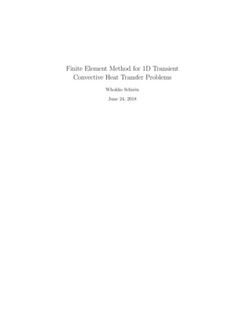
3RESULT AND ANALYSIS10For the system in Figure 3 we get the global stiffness matrix 1 1 00 1 2 1 0 K 0 1 2 1 ,00 1 1and 1 1Ka 00 12 100 12 1 ui0 uj0 1 ukul1 . The global damping matrix and force vector are assembled similarly. This wayof assembling the global systems of linear equations will be applied to all FEMin this work.It is now time to integrate with respect to time. The force vector f could bea function of time but that case will not be considered here and now, only a(t)and ȧ(t) are considered.3.1.2Discretisation in time of the 1D heat equation without convectionWe want to find a discretisation in time. We consider the temperature an attime tn as known, and let t be a finite time increment, then we are searchingfor the temperature an 1 at time tn 1 tn t, [9, pp. 494–495]. We also letτ be normalised time such that it is set to zero at time tn and is equal to t attime tn 1 . If t is the actual time then the time variable τ t tn , [5, p. 195].The shape functions with respect to time should be such that N̂n 1 at time nFigure 5: Visualisation of the time discretisation, Figure 18.1 in [9].and equal to zero at all other time steps, and N̂n 1 1 at time n 1 and equal
3RESULT AND ANALYSIS11to zero at all other time steps, as in [5, pp. 195–196]. Then the shape functionvector N̂ take the formhττ i,(0 τ t).N̂ 1 t tThe approximation of the temperature at the nodes, depending on time, thenisa(τ ) N̂n an N̂n 1 an 1 .Substituting for the shape functions gives the temperature with respect to timeas τ τ an an 1 .(12)a(τ ) 1 t tThe derivative of a(t) with respect to time isid h τ id h τ 1 an an 1dτ t dτ t11an an 1 t tan 1 an . tȧ(τ ) (13)Substituting (12) and (13) into (11) yields an 1 anττCKan Kan 1 f. Kan t t tNext we multiply by the weighting function w (τ ) and integrate over the timestep t to get Z tZ tZ tan 1 anτw (τ ) CKan dτdτ w (τ ) Kan dτ w (τ ) t t000Z tZ tτKan 1 dτ w (τ ) f dτ.w (τ ) t00We then divide the above expression by CR tR t τw (τ ) tdτan 1 an Kan 0R t tw (τ ) dτ0w (τ ) dτ to obtainR t!Kan 0which if0τw (τ ) tdτR t0w (τ ) dτ!Kan 1 f,R tτw (τ ) tdτΘ 0R t,w (τ ) dτ0could be rewritten as an 1 anC Kan ΘKan ΘKan 1 f. t(14)
3RESULT AND ANALYSIS12Assuming that an is a known temperature at time n we search for the temperature an 1 after a certain time has passed. Expanding the terms and collectinglike terms we get CC ΘK an 1 K (1 Θ) an f. t tAs an is a known temperature and the only unknown is an 1 , this could begeneralised asK an 1 f ,(15)whereC ΘK, t C K (1 Θ) an ff tK andZhNT ρcN dx,C 0ZK hBT AkB dx,0 hf NT Aq 0as before. Note that the matrices C and K are symmetric. Also remember thatthe force does not depend on time, therefore if we simplify the force vector westill get 1f Aq 1as in Section 3.1.1. In Section 3.2 we will make a finite element implementationof (15) to study the heat transfer without convection.3.1.3Discretisation in space of the 1D heat equation with convectionIn this section we add convection to our one dimensional problem. This will leadto non-symmetrical stiffness matrices that can not be made symmetric with thestandard Galerkin weighting used in Section 3.1.1, [10, p. 14]. To find a solutionfor this we will first study an example to understand where the Péclet numbercomes from, we will then introduce another weighting function to take care ofthe problem with non-homogeneous stiffness matrices, [10, pp. 15–20].Symmetric matrices should not be an absolute necessity to find a solution forthe system of algebraic equations, but it simplifies the numerical computationsso that the system of algebraic equations is more efficiently solved by computers.It is therefore common to change weighting function so that symmetric matricesare obtained.
3RESULT AND ANALYSIS13Standard steady state FE formulationWe use the same approximations as in Section 3.1.1, that isu (x, t) Nav (x) Nc cT NT vT u Ba x v cT BT , x u Nȧ tand substitute into (10) to obtaincZThThZN ν̄Ba dx 0ZTThTB kBa dx N qN ρcNȧ dx 0h0ih!.0Remember that we let A 1 for the case with convection. As cT is a arbitraryvector we can eliminate it and are left with!Z hZ hZ hhihBT kB dx NT ν̄B dx a NT q .NT ρcNȧ dx 0000Observe that the expression in parentheses in front of a is non-symmetric asRe h NT ν̄B dx. Then,NT B is non-symmetric. Put the convection matrix K0e together with C, K and f as defined at the end of Section 3.1.2, weusing Kobtain e a f.Cȧ K K(16)This is the system that we want to solve and many solutions have been suggestedand considered to find a solution for the non-symmetric part. For simplicity wee as stiffness matrices even though they havewill refer to the matrices K and Kslightly different functions in our model.We want to find a solution to the problem with the non-symmetry and startby studying a simple example of the steady state version of (16). As done in [5,p. 183] we put the right hand side equal to zero, e a 0.K K(17)Assume that we have only two elements with length h, and u1 , u2 and u3 aregiven temperatures at the nodes 1, 2 and 3. From the definition of the stiffnesse we getmatrices K and K ekν̄ 1 11 1eeK K ,h 1 12 1 1the superscript e denotes that this is the stiffness for a local element. Weassemble the global stiffness matrix and (17) take the form 1 1 0 1 1 0u1 ν̄ke a 1 2 1 1 0 1 u2 0.K Kh20 1 10 1 1u3
3RESULT AND ANALYSIS14We then consider the middle row to assemble the equation for node 2 askν̄( u1 2u2 u3 ) ( u1 u3 ) 0,h2a formulation typical for the finite difference method. We multiply by h/k( u1 2u2 u3 ) ν̄h( u1 u3 ) 0.2kThe parameter P e ν̄h2k stem from the finite difference method and is calledthe element Péclet number, [10, p. 16], [5, p. 183]. Different values of the Pécletnumber have been studied, tested and compared to analytical solutions of theproblem. If Pe 0, i.e. if ν̄ 0, then we have a purely diffusive problem, andif Pe we have a purely convective problem [10, p. 18]. It has also beenobserved that if Pe 1 then the solution becomes unstable and no exact nodalvalues can be obtained [10, p. 19]. In the next Section we will study a solutionto this problem.Optimal steady state FE formulationUntil now we have used the approximation u (x, t) Na and the standardGalerkin weighting v (x) Nc. To solve the problem with non-symmetric stiffness matrix we will do as suggested in [10, p. 18] and change to a Petrov-Galerkintype of weighting function to find a solution for (16). This is possible as we havelinear shape functions. We start by studying the weight for a single node i, putυi (x) Ni αew i (x) ,where Ni is a shape function and we i (x) is such thatZ hhwe i (x) dx ,20the sign depend on the direction of the velocity ν̄. We will get back to theconstant α later in this Section.The weighting function could be chosen in many ways, but according to [10,p. 19] the most convenient way is to define υi asυi (x) Ni αh dNi(sign ν̄),2 dxiwhere we i (x) becomes h2 dNe i could be positivedx and sign ν̄ reminds us that wor negative depending on the direction of the velocity. Remember that it hasbeen observed that the solution becomes unstable if Pe 1, see the previousSection. According to [10, p. 19] and [2, p. 1393] it is possible to choose anoptimal value of α so that we get exact nodal values for all values of Pe, thisoptimal value is obtained if α αopt coth Pe 1. Pe
3RESULT AND ANALYSIS15To get the sign of ν̄ we multiply the second term of υ with γ ν̄/ ν̄ . The fullexpression for the weighting function is h dNυ(x) N αoptγ c2 dxor! ThdNh TTTTTTυ (x) cN αoptγ cN αopt B γ .2 dx2Observe that υ cT BT xas the second term of υ is a constant and therefore will be zero when we takethe derivative.We substitute for this new weighting function in (10), letting u u Ba Nȧ x tas always, this yields the following weak formulation, note that we have eliminated cT as before, Z h Z h h Th TTTN αopt B γ ρcNȧ dxN αopt B γ ν̄Ba dx 2200 hZ hh BT kBa dx NT αopt BT γ q .200u(x, t) NaThis could, as in Section 3.1.1, be reformulated as the finite element formulation e a f,Cȧ K K(18)with a different damping matrixZ hZ hhTC N ρcN dx αopt BT γρcN dx200 ρch 2 1h 1 1 αopt BT γρc,1 21164and conductivity matrixZK 0hBT kB dx kh 1 1 11 ,and the convection matrixZ hZ hhe KNT ν̄B dx αopt γBT ν̄B dx200 ν̄ν̄ 1 11 1 αopt γ. 2 1 12 1 1The discretisation, (18), is our discretisation in the spatial domain, next wesearch for a discretisation of (18) in the time domain.
3RESULT AND ANALYSIS3.1.416Discretisation in time of the 1D heat equation with convectionWe start by multiplying (18) with a time weighting function,Z tZ tZ t e a dτ w (τ ) Cȧ dτ w (τ ) K Kw (τ ) f dτ 0.00(19)0We use the same approximations as we did for the time discretisation in Section3.1.2, anττa(τ ) N̂a 1 t tan 1 ττ an an 1 1 t tand 1an1N̂a t tȧ(τ ) an 1 τan 1 an, tand substitute the approximations into (19) to yieldZ tZ ti h ττ an 1 anedτ an an 1 dτw (τ ) K K1 w (τ ) C t t t00Z tw (τ ) f dτ 0. 0R tIf we again divide throughout with 0 w (τ ) dτ and letR tτdτw (τ ) tΘ 0R t,w (τ ) dτ0then an 1 an e (an Θ (an 1 an )) f. K K tWe collect like terms and end up with CCee Θ K K an 1 (1 Θ) K K an f, t tCwhich is generalised asK an 1 f ,(20)where Ce Θ K K t C ef (1 Θ) K K an f. tK The system of linear equations (20) is the system that we will make a MATLABimplementation for in the next Section.
3RESULT AND ANALYSIS3.217Finite element implementationIn this section we are going to study the MATLAB implementations for heattransfer with and without convection and present the results.In the weak formulations (15) and (20), which we are going to make finiteelement models of, there is a parameter Θ that we have to choose. We usethe Galerkin type 2 scheme which is one of the possibilities given in [5, p. 197]and put w τ / t and calculate the integral (14). We find that Θ 2/3when w τ / t. We could have chosen w differently, the solutions will beunconditionally stable for 0.5 Θ 1 and for Θ 0 we get a conditionallystable solution which requires certain criteria to be fulfilled for the length of thetime step, [5, p. 197].The sets of parameter values used in the FE-models have been chosen toreflect how the analytic solutions, found in Section 3.4.1 and 3.4.2, are derived.This has been done to make it possible to make comparisons between the finiteelement implementations and the analytical solutions. For the FE-model for 1Dheat transfer without convection the following set of parameters has been used:length L π, heat conductivity k 5 10 13 , density ρ 1, heat capacityc 1 and total time T 1.7 1012 . For the model with convection we insteaduse: length L 1, heat conductivity k 1, density ρ 1, heat capacity c 1,convective velocity ν̄ 10 and total time T 0.2.MATLAB is a program built to handle matrix manipulations effectively.There are a lot of toolboxes available to be used together with MATLAB and inour implementation we use two functions from the CALFEM toolbox, namelyassem.m and SOLVE.m. The purpose of assem.m is to assemble element matrices, such as the stiffness matrices, into a global matrix. The order of theassembly is decided by a topology matrix called edof in which the degrees offreedom are specified. The function SOLVE.m solve systems of linear equationstaking stiffness matrices, load vectors and boundary conditions as input data.From executing the implementation found in Appendix A we get the plotsin Figure 6
model which we then do a discretisation on using the nite element method, this gives us a discrete solution. As a mathematical model we use the heat equation with and without an added convection term. We discretise the model using the Finite Element Method (FEM), this gives us a discrete problem. We