WIXLIB

THE MORTAR FINITE ELEMENT METHOD IN 2D:IMPLEMENTATION IN MATLABJ. Daněk 1 , H. Kutáková12Department of Mathematics, University of West Bohemia, Pilsen2 MECAS ESI s.r.o., PilsenAbstractThe paper is focused on the mortar finite element method for solving linearelliptic problems in 2D. The mortar finite element method is a nonconformingdomain decomposition technique tailored to handle problems posed on domainsthat are partitioned into independently triangulated subdomains. In the contribution we explained the principle and properties of the method. A significantpart of the paper is dedicated to the implementation of the mortar method inthe Matlab system. The numerical results are showing both the principle andthe possibility of practical use of the method.1IntroductionThe finite element method is applicable to a wide range of physical and engineering problemswhich can be described by means of partial differential equations. The mortar finite elementdiscretization is a discontinuous Galerkin approximation. The functions in the approximationsubspaces have jumps across subdomain interfaces and are standard finite element functionswhen restricted to the subdomains. The jumps across subdomains interfaces are constrainedby conditions associated with one of the two neighboring meshes so that a weak continuitycondition must be fulfilled. Because of the discontinuity on the interface we classify the mortarfinite element method as a nonconforming finite element method (see [6]).Mortar finite elements were first introduced in 1994 by Christine Bernardi, Yvon Madayand Anthony T. Patera in [1]. Our paper is focused on the mortar finite element method in twodimensions and its implementation in the Matlab system. Most of the literature describing themortar finite element method deal with the geometrically conforming partition, which is easier.Therefore, this paper is focused on the nonconforming case.2Mortar Finite Element MethodIn this section we briefly describe the mortar finite element method in two dimensions. LetΩ R2 be a polygonal computational domain. We decompose the domain into P nonoverlappingpolygonal subdomainsΩ P[Ωi ,Ωj Ωk for j 6 k,j, k 1, . . . , P.i 1The partition can be: Geometrically conforming – The intersection between two closure of any two subdomainsΩi Ωj , i 6 j is either an entire edge, a vertex or empty. Figure 1 shows an example ofthe partition. Geometrically nonconforming – All the other cases. See example of the nonconformingpartition in Figure 2.

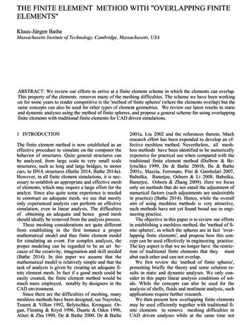
ΩΩ1Ω6Figure 1: Example of geometrically conforming partition of Ω into subdomains Ω i .ΩΩΩ1Ω1Ω7Ω5Figure 2: Example of geometrically nonconforming partition of Ω into subdomains Ω i .The subdomains Ωi form together a coarse mesh of the whole domain Ω. We discretizeeach subdomain by triangular elements known from the finite element method. The size of thetriangles can be chosen with regard to the problem. We use finer mesh in subdomains, wherebig changes in behaviour of the solution are expected, etc. The resulting triangulation can benonmatching across the interfaces of the subdomains, as you can see in Figure 4.We define the interface Γ between subdomains Ω i as a closure of the union of the parts ofthe boundaries of Ωi , i 1, . . . P , that are interior to ΩΓ Pi 1 ( Ωi \ Ω).(1)The interface can be considered also as a set of nodes, that belong to the boundary of at leasttwo subdomains.We denoteV h (Ω) V1h (Ω1 ) V2h (Ω2 ) · · · VPh (ΩP )(2)the space of mortar finite elements defined on Ω. We consider the low order basis functions, forexample the piecewise linear basis functions. V ih (Ωi ) is a finite element space in each subdomainΩi . Vih (S) is a restriction of functions from V h to a set S.For further analysis, we introduce some more notation. A main edge will represent a sideof a planar n-agle, see Figure 3. A square has four main edges, n-agle has n main edges. LetΓij be an open common edge or a part of an edge of two adjacent subdomains Ω i and ΩjΓij Ωi Ωj .(3)The edge Γij is a part of a main edge (or is a main edge) both of the subdomain Ω i and Ωj . Wechoose the main edge of one subdomain as a master (mortar) and the main edge of the secondsubdomain as a slave (nonmortar). We use a new notation: Mortar edge γ – If it belongs to a particular main edge of a boundary Ω i , we denote itγi . Nonmortar edge δ – If it belongs to a particular main edge of a boundary Ω j , we denoteit δj .

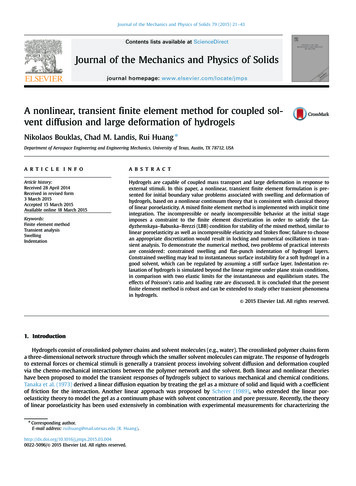
Figures 3 and 4 show examples of situations, that can occur on the interface. If we considergeometrically conforming partition of Ω, it is obvious, that for two subdomains Ω i and Ωj witha commom edge holds an equality γi Γij δj , or γj Γij δi (it’s important which edgeis chosen as a mortar), see Figure 4. The situation is more complicated in the nonconformingcase. There is arising a question, how to choose mortar and nonmortar edges. An example ofsuch a choice is in Figure 5. It can be proven that the partition always exists (see [3] or [6]).In term of a new notation we can write:Γ K[γm γn ,γk ,if m 6 n,m, n 1, . . . , K,(4)m, n 1, . . . , L,(5)k 1where K is the number of all mortar edges. Obviously alsoΓ L[δm δn ,δl ,if m 6 n,l 1where L is the number of all nonmortar edges.ΩΓijmain edge Ωimain edge ΩjΩiΩjγiδjFigure 3: Interface Γij of two subdomains Ωi and Ωj and signification of edges as mortar andnonmortar.ΩΓijΩiδiΩjγjFigure 4: Mortar edge γ and nonmortar edge δ on the interface Γ ij of two subdomains Ωi andΩj .It remains to solve the most important point of the method - the situation on the interfaceΓ. It’s necessary to join somehow the values of the searched function (we call it mortar function)

ΩΩΩ1Ω1Ω7Ω5Figure 5: Example of choice of mortar edges in geometrically nonconforming case (mortar edgesare blue).on the interface. Instead of a pointwise continuity we require fulfilment of a weak continuitycondition. The exact formulation will follow after some necessary definitions.Each nonmortar edge δl belongs to exactly one subdomain, we denote it Ω l . Let Γl be theunion of q parts of the mortar edges γ l,i which correspond geometrically to nonmortar edge δ lΓl q[(γl,i δl ).(6)i 1For each nonmortar edge δl we choose a space of test functions Ψ h (δl ), which is a subspaceof the space Vlh (δl ), that is a restriction of functions from V lh (Ωl ) to δl . So if we choose piecewiselinear basis functions, Vlh (Ωl ) will be a space of piecewise linear functions. Ψ h (δl ) will be arestriction of functions from Vlh (Ωl ) to δl with requirement that these continuous, piecewiselinear functions are constant in the first and last mesh intervals of δ l (see Figure 6). Otherpossibility how to establish the space of test functions is described in [7].Figure 6: Test functions on δl .We define the mortar projection on δl as πq1 ,q2 (ul ) : L2 (Γl ) Vlh (δl ). For two arbitraryvalues q1 and q2 and a function ul L2 (Γl ) it satisfiesZ(7)(ul πq1 ,q2 (ul ))ψ ds 0 ψ Ψh (δl ).δlThe condition means, that the jump of the mortar function across each nonmortar edge mustbe orthogonal (in L2 (Γl )) to the space of test functions defined on δ l . The condition is calledthe weak continuity condition or the mortar condition.

3Formulation of the Mortar Problem3.1Variational (Weak) Formulation of the Mortar ProblemLet us remind a variational (weak) formulation of a Poisson problem in two dimensions. Weneed to find a solution u W21 (Ω) of the Poisson equationu g1 4u fin Ω R2 ,(8)on ΩD , u g2 n(9)on ΩN ,where f L2 (Ω), g1 L2 ( ΩD ), g2 L2 ( ΩN ). The solution u W21 (Ω) must be from the setof admissible functionsVg {u W21 (Ω) : u g1 na ΩD in the sense of traces}(10)and for every test function v must satisfy v V,a(u, v) F (v)(11)whereV {v W21 (Ω) : v 0 on ΩD in the sense of traces}.Za(u, v) [grad u grad v] dΩ,F (v) ZΩf v dΩ Zg2 v dS.(12)(13)(14) ΩNΩWe can formulate the problem (8), (9) in terms of a decomposition of the domain Ω intosubdomains Ωi , i 1, 2, . . . , P and by using an appropriate mortar finite element space V h . Weappear from the weak formulation (11) of the problem (8), (9) and we rewrite it to the discreteform.We know, that Vih (Ωi ) W21 (Ωi ), i 1, . . . , P . Thus, we can writeaΓ (u, v) F Γ (v) v W21,0 (Ω).(15)aΓ (·, ·) is a bilinear form, which is defined as a sum of contributions from the particular subdomainsP ZXΓa (u, v) [grad u grad v] dΩi(16)i 1 ΩandF Γ (v) F (v) iZΩf v dΩ Zg2 v dS.(17) ΩNA variational (weak) formulation of the mortar problem represents such a task: Find u h V hwhich satisfiesaΓ (uh , vh ) F Γ (vh ) vh V h .(18)The existence and uniqueness of the solution of (18) follows i.a. from the Lax-Milgram lemma.

3.2Mixed Formulation of the Mortar ProblemFirst, we present some findings relating to dual spaces. We know, that V ih (Ωi ) W21 (Ωi ). A1/2restriction of a mortar function u to a nonmortar edge δ l belongs to the space W2 (δl ). The1/2space of test functions Ψh (δl ) can then be a subset of the dual space of space W 2 (δl ) with 1/2respect to the L2 inner product, thus Ψh (δl ) W2(δl ).For introduction of a mixed formulation we use the mortar condition (7), whose satisfactionis demanded on the interface. We denote [u l ] the jump of uh V h across δl . The test functionsfrom the mortar condition can be considered as Lagrange multipliers. A function u belongs tothe space V h if and only if for all the nonmortar edges δ l and for all the Lagrange multipliersµl , which form a basis of Ψh (δl ), holdsZ[ul ]µl ds 0.(19)δl1/2From the first paragraph of this subsection results, that [u l ] W2 (δl ). Lagrange multiQQ 1/2 1/2pliers µl must then be from the dual space W2(δl ). Let M h l Ψh (δl ) l W2(δl ) andhµh M , where µh (µl )l 1:L , L is the number of nonmortar edges. We define a bilinear formb(uh , µh ) L ZX[uh ]µl ds.(20) µh M h .(21)l 1 δlA function uh is a mortar function if and only ifb(uh , µh ) 0We can rewrite the discrete problem (18) to the mixed formulation: Find a couple (u h , λh ) V h M h which satisfiesaΓ (uh , vh ) b(vh , λh ) F Γ (vh )b(uh , µh ) 0 vh V h , µh M h .(22)As well as in other mixed formulations, it is important to satisfy the Brezzi-Babuškacondition (see [7]) also in formulation (22). This is important for the existence of the solutionand for the error estimate.4Implementation of the Mortar Finite Element MethodWe describe briefly the key points of the implementation of the mortar finite element methodin the Matlab system. We started from the program [4], which deals with the conformingpartition of the computational domain into squares and rectangles, whose sides are parallelto the coordinate axes. The generalization of the program to the nonconforming case is nota trivial task. Our program solves the Poisson or Laplace equation in two dimensions withDirichlet boundary condition and can deal with polygonal computational domains, that can bedivided into general polygonal convex subdomains. Since the conforming partition is a specificcase of the nonconforming partition, it’s obvious, that the program can handle with conformingcase also.The input data are the geometry of the computational domain, the right hand side and theDirichlet boundary condition. The geometrical data contain informations about the subdomains- each subdomain and its triangulations is inscribed with a triplet of matrices p, e, t representingmatrices of points, edges and triangles. It’s necessary to save the information on the mutual