WIXLIB

N. Bouklas et al. / J. Mech. Phys. Solids 79 (2015) 21–4323solvent, defined as the number of solvent molecules per unit volume of the polymer in the reference configuration. In thisformulation, the free energy consists of two parts, one for elastic deformation of the polymer network (Ue) and the other forpolymer-solvent mixing (Um). The free energy is proportional to the thermal energy kBT, with Boltzmann constant kB andtemperature T. In addition, it depends on the effective number density of polymer chains in the dry state (N), the molecularvolume of the solvent (Ω ), and the Flory parameter ( χ ) for the polymer–solvent interaction.In previous works (e.g., Hong et al., 2008; Zhang et al., 2009), both the polymer and the solvent were assumed to beincompressible. As a result, the volumetric strain of the hydrogel is solely related to the solvent concentration, whichimposes a constraint on the deformation gradient. Such a constraint is lifted in the present study to allow compressibility byadding a quadratic term into the elastic free energy, namelyUe (F , C) 1KNkB T [FiK FiK 3 2 ln(det(F))] (det(F) 1 ΩC)222(2.4)where K is a bulk modulus with the same unit as NkB T (shear modulus). It is expected that the behavior of the hydrogelpredicted by the modified free energy function approaches that by the original theory when the bulk modulus is sufficientlylarge (i.e., K NkBT ). Note that the elastic free energy in (2.4) introduces a coupling between deformation gradient andsolvent concentration at the constitutive level.The nominal stress and chemical potential of the solvent in the hydrogel are obtained from the free energy densityfunction assiJ μ U NkB T (FiJ αHiJ ) FiJ(2.5) (1 ΩC) χ UΩC ΩK (det(F) 1 ΩC) kB T ln C(1 ΩC)2 1 ΩC(2.6)whereα 1K(det(F) 1 ΩC), det(F)NkB T(2.7)1HiJ 2 eijk eJKL FjK FkL .(2.8)Mechanical equilibrium is assumed to be maintained at all time during the transient process, which requires that siJ X J bi 0 in V0siJ NJ Ti on S0(2.9)(2.10)where bi is the nominal body force (per unit volume), V0 is the volume in the reference configuration, NJ is unit normal onthe surface of the reference configuration, and Ti is the nominal traction on the surface. In addition, prescribed displacements can be specified as essential boundary conditions.On the other hand, the gel has not reached chemical equilibrium in the transient stage. The gradient of chemical potential drives solvent migration inside the gel. By a diffusion model (Hong et al., 2008), the true flux of the solvent in thecurrent state is given byjk cD μkB T xk(2.11)where c is the true solvent concentration defined in the current configuration, which is related to the nominal concentrationas c C /det(F), and D is a constant for solvent diffusivity.With respect to the reference configuration, the nominal flux by definition is related to the true flux as: JK NK dS0 jk nk dS ,where nk is the unit normal in the current configuration and the differential areas dS0 and dS are related asFiK ni dS det(F) NK dS0 . The nominal flux can then be obtained from Eq. (2.11) asJK det(F) XK μjk MKL xk XL(2.12)which defines a nominal mobility tensor:MKL DC XK XL .kB T xk xk (2.13)

24N. Bouklas et al. / J. Mech. Phys. Solids 79 (2015) 21–43By mass conservation, a rate equation for change of the local solvent concentration is obtained as JK C r in V0 t XK(2.14)where r is a source term for the number of solvent molecules injected into unit reference volume per unit time. Thechemical boundary condition for the gel in general can be a mixture of two kinds, i.e., S0 Si Sμ , where the solvent flux isspecified on Si and the chemical potential is specified on Sμ .3. Finite element formulationThis section presents a finite element formulation based on the nonlinear theory in Section 2, starting from the strongform of the governing equations and initial/boundary conditions, to the weak form of the problem, and then to the discretization and solution procedures.As the strong form of the initial/boundary-value problem, the governing field equations in (2.9) and (2.14) are complemented by a set of initial and boundary conditions. The initial conditions are typically described by a displacement field(u x X ) and chemical potential:u t 0 u0(3.1)μ t 0 μ0(3.2)Relative to the dry state (μ ), the initial displacement field can be prescribed for a homogeneous deformationcorresponding to a constant chemical potential (e.g., μ0 0).At t 0 , boundary conditions are applied. The mechanical boundary condition can be prescribed with a mixture oftraction and displacement:siJ NJ Ti or ui u i on S0(3.3)Similarly, the chemical boundary condition is prescribed asJK NK i or μ μ on S0(3.4)where i is the surface flux rate (number of solvent molecules per unit reference area per unit time, positive inward) and μ̄ isthe surface chemical potential depending on the surrounding environment.Since the chemical boundary conditions for gels are often specified in terms of chemical potential or diffusion flux(proportional to the gradient of chemical potential), it is convenient to use the chemical potential (instead of solventconcentration) as an independent variable in the finite element formulation. For this purpose, we re-write the free energydensity as a function of the deformation gradient and chemical potential by Legendre transform: U (F , μ) U (F , C) μC(3.5)Similar to Eqs. (2.5) and (2.6), we havesiJ (F , μ) U FiJC (F , μ ) (3.6) U μ(3.7)which yield the same constitutive relationships but the solvent concentration is now given implicitly by solving a nonlinearalgebraic equation in (2.6). We also note that the continuity requirement for the nonlinear finite element formulationremains C0 by using the chemical potential instead of the concentration as a nodal degree of freedom.3.1. Weak formThe solution to the initial/boundary-value problem consists of a vector field of displacement and a scalar field of chemicalpotential, u (X , t) and μ (X , t), which are coupled and evolve concurrently with time. The weak form of the problem isobtained by using a pair of test functions, δ u(X) and δμ (X), which satisfy necessary integrability conditions. Multiplying Eq.(2.9) by δui , integrating over V0 , and applying the divergence theorem, we obtain that V0siJ δui, J dV V0bi δui dV S0Ti δui dS(3.8)

N. Bouklas et al. / J. Mech. Phys. Solids 79 (2015) 21–4325Similarly, multiplying Eq. (2.14) by δμ and applying the divergence theorem for the volume integral, we obtain that V0 CδμdV t V0JK δμ, K dV VrδμdV 0 SiδμdS(3.9)0Hence, the weak form of the problem statement is to find u (X , t) and μ (X , t) such that the integral Eqs. (3.8) and (3.9) aresatisfied for any permissible test functions, {δ u, δμ} .3.2. Time integrationA backward Euler scheme is used to integrate Eq. (3.9) over time: V0C t Δt C tδμ dV Δt V0JKt Δt δμ, K dV Vr t Δtδμ dV 0 Sit Δt δμ dS(3.10)0where the superscripts indicate quantities at the current time step (t Δt) or the previous step (t). The implicit backwardEuler integration scheme is first order accurate and allows for improved numerical stability compared to the explicit forwardEuler integration.Combine Eq. (3.10) with Eq. (3.8) and rearrange to obtain V (siJ0 )δui, J Cδμ Δt JK δμ, K dV V (bi δui rΔt δμ C tδμ)dV S00Ti δui dS SiΔt δμ dS(3.11)0where the superscript (t Δt) is omitted for all the terms at the current time step andprevious time step.Ctis the solvent concentration at the3.3. Spatial discretizationNext the displacement and chemical potential are discretized through interpolation in the domain of interest:u N uun and μ N μμnNuNμ(3.12)unμnwhereandare shape functions,andare the nodal values of the displacement and chemical potential, respectively. The test functions are discretized in the same wayδ u N uδ un and δμ N μδμn(3.13)The stress, solvent concentration, and flux are evaluated at integration points, depending on the gradients of the displacement and chemical potential via the constitutive relations. Taking the gradient of Eq. (3.12), we obtain that u F I N uun Buun(3.14a) μ N μμn B μμn(3.14b)where Bu and B μ are gradients of the shape functions. In this formulation we have allowed the use of different shapefunctions to interpolate displacement and chemical potential.Before proceeding to choose a type of interpolation for displacement and chemical potential, it is important to considerthe nearly incompressible behavior of a hydrogel at the instantaneous limit (t 0). In linear elasticity, at the incompressiblelimit, a finite element method with displacement as the only unknown would fail to converge to the true solution. Thus amixed finite element method with both displacement and pressure as the unknown fields must be employed (Hughes,1987). In order for the mixed method to produce numerically stable results, the LBB condition must be satisfied (Babuška,1971; Brezzi, 1974). This is ensured by the appropriate choice of shape functions for interpolation of the displacement andpressure. Elements with shape functions of equal order do not satisfy the LBB condition and hence produce numericaloscillations. A family of elements that satisfy the LBB condition are the Taylor–Hood elements (Taylor and Hood, 1973),where interpolation for pressure is one order lower than for displacement. However, the combination of zero-order constantpressure and first-order linear displacement results in spurious pressure modes (Sussman and Bathe, 1987). Thus, the lowestorder Taylor–Hood element that produces stable results combines first-order linear interpolation for pressure and secondorder quadratic interpolation for displacement.Similar numerical issues have been noted in linear poroelasticity when the instantaneous response is nearly incompressible. Vermeer and Verruijt (1981) first proposed a stability condition for the poroelastic consolidation problem,where the time step had to be larger than a proposed value. It was established later that this numerical instability was dueto the use of unstable elements in the LBB sense (Zienkiewicz et al., 1990). Extensive discussions about the numerical issuesfor solving Biot’s consolidation problem with mixed finite element methods have been presented by Murad and Loula (1992

26N. Bouklas et al. / J. Mech. Phys. Solids 79 (2015) 21–43and 1994), Wan (2002), and Phillips (2005). In the case of a poroelastic medium with incompressible or nearly incompressible constituents, numerically oscillating solutions for the pore pressure field are obtained at the initial stages ofthe evolution process when the shape functions for the displacement and pore pressure do not satisfy the LBB condition. Asthe equations turn from elliptic to parabolic in the transient stage, the diffusion process is known to regularize the oscillating solution and the oscillations would eventually vanish after a sufficiently long time.It has been shown that the nonlinear continuum theory proposed by Hong et al. (2008) reduces to Biot’s linear poroelasticity theory for small deformation of an isotropically swollen gel (Bouklas and Huang, 2012). Thus, similar numericalissues are to be expected for the finite element method in the present formulation when the instantaneous response isnearly incompressible (K NkBT ). In the continuum theory for hydrogels, chemical potential plays the role of pore pressurein linear poroelasticity. To satisfy the LBB condition, the shape function for chemical potential must be one order lower thanfor the displacement in the mixed finite element method. Otherwise, numerical oscillations would be significant and instantaneous response of the hydrogel may not be correctly predicted, as shown in Section 4. The necessity to employ astable combination of the shape functions was first noted by Wang and Hong (2012) in their study on visco-poroelasticbehaviors of polymer gels.In the present study, we have implemented the Taylor–Hood elements with quadratic shape functions for the displacement and linear shape functions for the chemical potential. For comparison, equal-order elements with quadraticshape functions for both displacement and chemical potential are also implemented. Regardless of the choice of shapefunctions, the same steps are followed to calculate the nominal stress (s ), nominal concentration (C ) and flux ( J ) at theintegration points, to numerically integrate the weak form over each element, and then to assemble globally to form asystem of nonlinear equations. In particular, the nominal concentration C is first calculated at each integration point bysolving Eq. (2.6) with the interpolated chemical potential and the displacement gradient. A one-dimensional Newton–Raphson method is implemented to solve the nonlinear algebraic equation. Subsequently, the nominal stress is calculated byEq. (2.5) and the flux is calculated using Eq. (2.12).After the spatial discretization, invoking the arbitrariness of the test functions, the weak form in Eq. (3.11) can be expressed as a system of nonlinear equations,n (d ) f(3.15) un where d n . More specifically, the individual contributions to Eq. (3.15) are μ niu,M Vn μ, M V ( CN μ,M ΔtJK BKμ,M ) dVf iu,M V0siJ B uJ ,M dV(3.16a)00bi N u, MdV S0Ti N u, MdSf μ, M V (rΔt C t)N μ,MdV S00iΔtN μ, MdS(3.16b)where the superscript M refers to the node and the subscript in B uJ refers to the direction in which the derivative is taken.3.4. Newton–Raphson methodThe system of nonlinear equations in (3.15) are solved iteratively using the Newton–Raphson method at each time step.Noting that the right hand side of the equations only consists of known quantities, the residual in each iteration can becalculated asRi f n (di )(3.17)where di represents the solution at the ith iteration. The correction to the solution is then calculated as nΔdi d 1 Ridi (3.18)with which the nodal unknowns are updated for the next iteration as di 1 di Δdi . The iteration repeats until a suitablelevel of convergence is reached, both in terms of the nodal corrections, ‖Δd‖ 2 (Δdj ) , and the residual, ‖R‖ In particular, Eq. (3.18) requires calculation of the tangent Jacobian matrix at each iteration, namely2 (Rj ) .

N. Bouklas et al. / J. Mech. Phys. Solids 79 (2015) 21–43 n ddi K uu K uμ K μu K μμ 27(3.19)where for each pair of nodes (N , M ) and degrees of freedom (i, k):Kikuu,NM VB Ju,N 2UBLu,M dV FiJ FkL(3.20a)Kiuμ,NM VB Ju,N 2U μ, MN dV FiJ μ(3.20b)Kiμu, NM00 2 N μ, N U B u, MJ μ FiJ 2 F 1 UU 1 1Kk 1 dV FKkFLl FLl V0 μ FiJ D μ, N μ FiJNMu,N,μ μ BL BJ BK Δt 1kBT U 1 F Ll FKk Fμ iJ K μμ, NM V0 2 N μ . N U N μ, M2 μ dV D μ,N 2U 1 1 N μ,N μ, M U 1 1 μ,M tBFFBNFFB Δ μ Kk LlKk LlLL kB T K μ2 μ (3.20c)(3.20d)We notice that the derivatives of the mobility tensor in Eqs. ((3.20c) and (3.20d)) break the symmetry of the tangentmatrix. For a consistent Newton–Raphson method, a non-symmetric solver has to be implemented to achieve quadraticconvergence of the iterative procedure. Alternatively, a symmetric tangent Jacobian matrix may be used as an approximation withKiμu,NM VK μμ, NM V0 2 N μ, N U B Ju,M dV μ FiJ 2 N μ . N U N μ, M Δt D B μ, N U F 1F 1B μ, M dVKk Ll L K 2 μkBT μ0 (3.21a)(3.21b)so that the standard symmetric solver can be employed for the ease of computation. However, if the mobility tensor isupdated throughout the iterative process, the use of the inconsistent symmetric tangent matrix would lead to loss of thequadratic convergence, although the scheme remains fully implicit and unconditionally stable. On the other hand, if themobility tensor is fixed at the previous time step, the tangent matrix would be consistently symmetric and hence thequadratic convergence would be maintained. In this case, however, the time integration is partly explicit with the forwardEuler scheme for the mobility tensor. As a result, the time step has to be chosen appropriately to ensure stability. In thepresent study, both methods with the symmetric tangent matrix have been implemented, and both yield convergent resultsfor the specific problems considered.Fig. 1. Schematic of a hydrogel layer attached to a rigid substrate. Three types of boundary conditions (S1, S2, and S3) are indicated for the finite elementanalysis.

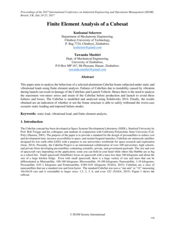
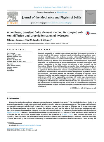
28N. Bouklas et al. / J. Mech. Phys. Solids 79 (2015) 21–434. Swelling of a hydrogel layerAs the first example, we consider constrained swelling of a hydrogel layer attached to a rigid substrate (Fig. 1). The sameproblem has been studied previously by both linear and nonlinear theories (Bouklas and Huang, 2012), which provides abenchmark for the finite element method developed in this study. A two-dimensional finite element (2D-FE) model is usedto simulate swelling of the hydrogel layer. As shown in Fig. 1, three types of boundary conditions are imposed onto thesimulation box: the surface (S1) is traction free and in contact with an external solvent so that μ X2 H 0; the bottom (S2) isattached to the substrate so that Δu X2 0 0(fixed displacement, Δu u u0 ) and J2 0 (zero flux); the two sides (S3)X2 0are subject to the symmetry conditions with Δu1 X1 0, a 0, s21 X1 0, a 0 and J1 0, where a is the length of the siX1 0, amulation box. The initial condition is set by a homogeneous swelling ratio λ0 corresponding to an initial chemical potential,μ0, which can be determined analytically (Appendix A). Relative to the dry state, the initial displacement is: u0 λ0 X X .For convenience, dimensionless quantities are used as follows: all lengths are normalized by the dry-state thickness of thehydrogel (H ), time is normalized by the characteristic diffusion time, τ H 2/D , stresses are normalized by NkB T , chemicalpotential by kB T , and solvent concentration by Ω -1.4.1. Numerical stabilityTo illustrate the issue of numerical stability, we compare the results from two types of spatial interpolation (Fig. 2). First,using eight-node quadrilateral elements with equal-order biquadratic interpolation for both the displacement and chemicalpotential (8u8p), the numerical results show significant oscillations at the early stage (Fig. 3), which decay over time andeventually vanish. This is expected because the 8u8p elements with equal order interpolation violate the LBB condition.Here, a relatively large bulk modulus is used, K 103NkB T , to simulate a hydrogel with nearly incompressible constituents.The simulation domain is a square in the reference and initial states (a/H¼1) and is discretized by a uniform mesh with thenumber of elements along each side ne 20. A 3 3 Gauss integration scheme is employed for full integration. The timestep is small at the early stage with Δt/τ 10 5 and it is gradually increased until the hydrogel reaches equilibrium.It is found that the decay of the numerical oscillation depends on the element size. The maximum oscillation occurs inthe first layer of the elements below the surface, with an averaged amplitude, Amax (μ″ 2μ′)/4 , where μ′ and μ″ are theFig. 2. Two types of quadrilateral elements: an equal-order eight-node element (8u8p) and a Taylor–Hood element (8u4p).Fig. 3. Numerical oscillations of the chemical potential in the early stage of constrained swelling for a hydrogel layer with NΩ 10 3, χ 0.4 , K 103NkB T ,and λ0 1.4 , using the 8u8p elements with ne ¼ 20.

N. Bouklas et al. / J. Mech. Phys. Solids 79 (2015) 21–4329Fig. 4. The amplitude of numerical oscillation in the chemical potential as a function of time, using different numbers of 8u8p elements. The time isnormalized by the diffusion time scale for the layer thickness in (a) and the time scale corresponding to the element size in (b).Fig. 5. Numerical oscillations of the chemical potential at t/τ 10 4 for hydrogels with different bulk moduli, using 8u8p elements. The other parametersare: NΩ 10 3, χ 0.4 , λ0 1.4 , and ne ¼ 20.chemical potentials at the second and third layers of nodes, respectively; the chemical potential is zero for the surface nodes(first layer) by the boundary condition. In Fig. 4, the oscillation amplitude Amax is plotted versus time normalized by twodifferent time scales, τ H 2/D and τe he2/D , where he is the element size (he H /ne ). The oscillation decays faster withrespect to t/τ when using smaller elements. With respect to t/τe , however, the oscillation amplitude evolution curves collapse, suggesting that the numerical solution becomes stable when t/τe 104 . Therefore, by red

The present study aims to develop a transient finite element method for large deformation of hydrogels based on a nonlinear continuum theory. Previously, finite element methods for equilibrium analyses of hydrogels have been developed (Hong et al., 2009a; Kang and Huang, 2010a), without considering the diffusion kinetics. More recently, several im-