Transcription
ϕπϕπFiPyA Finite Volume PDE Solver Using PythonD. Wheeler, J. E. Guyer & J. A. Warrenwww.ctcms.nist.gov/fipy/Metallurgy Division &Center for Theoretical and Computational Materials ScienceMaterials Science and Engineering Laboratory1
ay,ines andation of allfreezes towere to lookstrongm, but isu were able towerfulhat looks liketo each other.ndrites. Thet" of dendrites in a metal would look likeMotivationPDEs are ubiquitous in Materials Science problemsSolve PDEs in weird and unique waysEasy to pose problemsEasy to customizeword "dendron", which means a tree.often describe the form and structure ofure to left), with a main branch or trunk,h grow smaller side branches, and sobranches grow into each other and thereThe figure toa metal. Inny thousands,s mostdendrites aret and weldedDon’t care about numerical methodsis, howd or stretch itunder whatout or rusts.conductor of electricity. The dendritesother, and what's the best way to do thecation profoundly influences a material'sϕϕπ
What is FiPy?FiPy is a computer program written in Python to solve partial differentialequations (PDEs) using the Finite Volume methodPython is a powerful object oriented scripting language with tools fornumericsThe Finite Volume method is a way to solve a set of PDEs, similar to theFinite Element or Finite Difference methodsϕϕπ
Why a common code?Many interface motion codes for solving Materials Science problems atNIST.Phase Field for solidification and meltingPhase Field for grain boundary motionPhase Field for elasticityPhase Field for electrochemistryLevel Set code for electrochemistryetc Need for code homogeneityInstitutional memory is lost with constant rewriting of codesNeed for preservation and reuseLeverage different skill setsϕϕπ
DesignImplement interface trackingPhase Field, Level Set,Volume of Fluid, particle trackingObject-oriented structureEncapsulation and InheritanceAdapt, extend, reuseTest-based developmentOpen SourceCVS and compressed source archivesBug tracker and mailing listsHigh-level scripting languagePython programming languageϕϕπ
Design: test-based development485 major tests, comprising thousands of low-level testsTests are documentation (and vice versa)298Module fipy.variables.variablege (self, other )Test if a Variable is greater than or equal to another quantity a Variable(value 3) b (a 4) b(Variable(value 3) 4) b()0 a.setValue(4) b()1 a.setValue(5) b()1getitem (self, index )“Evaluate” the variable and return the specified element a Variable(value ((3.,4.),(5.,6.)), unit "m") "4 m"ϕϕπ
Design: test-based development485 major tests, comprising thousands of low-level testsTests are documentation (and vice versa)Running main .Variable. gt . docTrying: a Variable(value 3)Expecting: nothingokTrying: b (a 4)Expecting: nothingokTrying: bExpecting: (Variable(value 3) 4)okTrying: b()Expecting: 0okTrying: a.setValue(5)Expecting: nothingokTrying: b()Expecting: 1ok0 of 6 examples failed in main .Variable. gt . docϕϕπ
! "# ! "# !"#Finite Volume MethodtransientSolve a general PDEdiffusionsource 1 κ1mT) φ forarctanon2 (φ,a givendomaina field(κφ2T )2π a11 a12 (ρφ)b1 · (Γ φ) [ · (Γi )]n φ . . · (#uφ) Sφφ1 0 !"# b2 .aaφ21222! t"# ! "# !"# !"# thsource transientconvectiondiffusion. . n order diffusion. . . .%%%%% bn.φn (ρφ)dV Γ(#n · φ) dS Γn (#n · · · · ).dS a nn (#n · #u)φ dS Sφ dV 0!V t"#transient !S"#diffusion S! (ρφ) "# !S"# ! V "#sourceconvection · ( uφ) · (Γ φ) Sφ'()*'()* t'()*' () *nth order diffusiontransient&convectiondiffusionsource &ρφV (ρφV )old & [(#n · #u)Aφ]face V [ΓA#n · φ]face [ΓA#n · {· · · }]face (ρφ) tfaceface( facedV n· u)φdS Γ( n · φ)"#dS S!φ!"# !"# !"# !domain ttransient' V diffusion()transient*'S()*nth order diffusionconvection'Sso()convection* ' V ()soudiffusion,ρφV (ρφV )old , [( n · u)Aφ]face [ΓA n · φ]face tfaceface'()* '()* '()*ϕϕπ
m2 (φ, T ) φ 1 κ1 arctan (κ2 T )2πFinite Volume MethodSolve (ρφ)n PDE· (Γ φ) [ · (Γdomain a· (#uφ) i )] φ forφ Sφ 0a generalonagivenfield t! "# ! "# ! "# ! "# !"# transientdiffusionadiffusiona12 convection source nth orderIntegratePDE overarbitrarycontrol11 volumesφ1b1 . % φ2 % b2 %%% a21 a22 (ρφ) n (#n · ·. ·. · ) dS. . (# dS. S dV Γ(#n · φ) dS Γn·#u)φ 0. .φ dV. . V . t. . ! S ."#! V "# !S"# ! S "# ! "# sourcebntransientconvection φndiffusionnth order diffusion . . ann (ρφ)&&ρφV (ρφV )old & · ( · (Γ φ) faceSφ V Sφ [ΓA#n · φ]face [ΓA#n · {··u·φ)}]face[(#n · #u)Aφ] t t'face() * ' () * ' face() * '()*faceconvection!"# !"# transient!"# !diffusion"# source !"# transientdiffusion 'Vnth order diffusion sourceconvection (ρφ)dV v contro ( n · u)φ dS Γ( n · φ) dS Sφol tlu()* 'mSe()* 'S()* ' V ()transientconvectionsoudiffusion,ρφV (ρφV )old , [( n · u)Aφ]face [ΓA n · φ]face tfaceface'()* '()* '()*ϕϕπ
· (Γ φ) [ · (Γi )]n φ · (#uφ) Sφ 0! t"# ! "# !"# ! "# !"# Finite Volume Methodtransientnth order diffusiondiffusionconvectionsourceSolve a generalPDE on a%given domain for a% field φ%% (ρφ) dV Γ(#n· φ)dS Γ(#n· ···)dS (#n·#u)φdS Sφ dV 0 naaIntegratePDEoverarbitrarycontrolvolumes1112 tSVφ! V "# !S"# !S"# !"# !"# b11 . .convection φ sourcetransient b2 nth orderdiffusionEvaluate PDEdiffusionover polyhedralcontrolvolumesaa21222 . . . . . . old &&&ρφV (ρφV ) [ΓA#n · φ]face [ΓA#n · {· · ·.}]. face [(#n ·φ#un)Aφ]face bVn Sφ 0. tannfacefaceface%!"#transient !"#diffusion !"#'V!"# !"# sourceconvectionnth order diffusion (ρφ) · ( uφ) · (Γ φ) Sφ' t() * ' () * ' () * '()*transient convection diffusionsource (ρφ)dV ( n · u)φ dS Γ( n · φ) dS Sφfa tcevertex()* ' S ()* 'S()* ' V ()transientcellconvectionsoudiffusion,ρφV (ρφV )old , [( n · u)Aφ]face [ΓA n · φ]face tfaceface'()* '()* '()*ϕϕπ
Finite Volume MethodSolve a general PDE on a given domain for a field φ a11 volumesa12Integrate PDE over arbitrary controlφ1b1 . φ2 b2 Evaluate PDE over polyhedral controlvolumesaa2122 . . . . . Obtain a large coupled set of linearequations. in φ . φφ. n bn . aa11 a12nn φ1b1 . a11 a12 . φ2 b2 aa2122φb11 (ρφ) . .S . φ. 2·. ( uφ). . · (Γ φ) a21 a22 . . φb.2 ' * '()* '()*(). t.* . . ' () .sourcediffusion. .transient. . convection . . φnbn .ann .φbnn. (ρφ) . anndV ( n · u)φ dS Γ( n · φ) dS Sφ (ρφ) t uφ) * '·S(Γ φ) Sφ* ' V ()VS · ( '()*'()()' () * ' () * '()* (ρφ) t'()* ·( uφ) · (Γ φ) onvection* ' () * '()*transient' t() * ' ()sourceconvection diffusion transient (ρφ)old,ρφV (ρφV) n ·[( dV ,( un)φdS Γ( n· φ)dS Sφ · u)Aφ] [ΓA n· φ]faceface (ρφ) tSV t· u)φ*dS ' S ()' V ( n()*'()*'()dV Γ( n· φ)dS SdVφfaceface t()*VS ()'()*' 'transient()** 'convection'S()** diffusion' V' () *() ϕ sourcϕπ
Diffusion Example φ · ( φ) 0 t!"# ! "# # create a meshtransient# create a field variable · (#uφ) · ( φ) 0! "# ! "# # create the equation termsdiffusionconvection# create the equationdiffusionφ x 0 0φ x L 1# create a viewer# solveτφ φ α2 2 φ φ(1 φ)m2 (φ, T ) t T φ2 DT T t t! "# transient! "# diffusionm2 (φ, T ) φ !"#source 1 κ1 arctan (κ2 T )2π (ρφ) · (Γ φ) [ · (Γi )]n φ · (#uφ) Sφ! t"# ! "# !"# ! "# !"# ϕϕπ
Diffusion Example φ · ( φ) 0 t!"# ! "# # create a meshtransientdiffusionL nx * dx · (#uφ) · ( φ) 0"# ! "# from fipy.meshes.grid2D import! Grid2Dconvectiondiffusionmesh Grid2D(nx nx, dx dx)φ x 0 0# create a field variableφ x L 1# create the equation# create a viewer# solveτφ φ α2 2 φ φ(1 φ)m2 (φ, T ) t T φ2 DT T t t! "# transient! "# diffusionm2 (φ, T ) φ !"#source 1 κ1 arctan (κ2 T )2π (ρφ) · (Γ φ) [ · (Γi )]n φ · (#uφ) Sφ! t"# ! "# !"# ! "# !"# ϕϕπ
Diffusion Example φ · ( φ) 0 t!"# ! "# # create a meshtransientdiffusion · (#uφ) · ( φ) 0! "# ! "# # create a field variablefrom fipy.variables.cellVariableconvectionimport CellVariablediffusionvar CellVariable(mesh mesh, value 0)φ x 0 0φ x L 1def centerCells(cell):return abs(cell.getCenter()[0] - L/2.) L/10. φ t T φ2 DT T t tvar.setValue(value 1., cells centerCells))τφ mesh.getCells(filter α2 2 φ φ(1 φ)m2 (φ, T )# create the equation# create a viewer# solve! "# transient! "# diffusionm2 (φ, T ) φ !"#source 1 κ1 arctan (κ2 T )2π (ρφ) · (Γ φ) [ · (Γi )]n φ · (#uφ) Sφ! t"# ! "# !"# ! "# !"# ϕϕπ
Diffusion Example φ · ( φ) 0 t!"# ! "# # create a meshtransientdiffusion · (#uφ) · ( φ) 0! "# ! "# # create a field variable# set the initial conditionsconvectiondiffusiondef centerCells(cell):return abs(cell.getCenter()[0]- L/2.)φ x 0 0 L/10.φ x L 1var.setValue(value 1., cells mesh.getCells(filter centerCells))# create the equation# create a viewer# solveτφ φ α2 2 φ φ(1 φ)m2 (φ, T ) t T φ2 DT T t t! "# transient! "# diffusionm2 (φ, T ) φ !"#source 1 κ1 arctan (κ2 T )2π (ρφ) · (Γ φ) [ · (Γi )]n φ · (#uφ) Sφ! t"# ! "# !"# ! "# !"# ϕϕπ
Diffusion Example φ · ( φ) 0 t!"# ! "# # create a meshtransient# create a field variable · (#uφ) · ( φ) 0! "# ! "# # create the equationdiffusionconvectiondiffusionfrom fipy.terms.transientTerm import TransientTermφ x 0 0φ x L 1from fipy.terms.implicitDiffusionTerm import ImplicitDiffusionTerm## equivalent forms φ## eq (TransientTerm() 1))τ ImplicitDiffusionTerm(coeff α2 2 φ φ(1 φ)m (φ,T)φ2 t## eq TransientTerm() - ImplicitDiffusionTerm(coeff 1) T φ2 DT T eq (TransientTerm() - ImplicitDiffusionTerm(coeff 1) 0) t t# create a viewer# solve! "# transient! "# diffusionm2 (φ, T ) φ !"#source 1 κ1 arctan (κ2 T )2π (ρφ) · (Γ φ) [ · (Γi )]n φ · (#uφ) Sφ! t"# ! "# !"# ! "# !"# ϕϕπ
Diffusion Example φ · ( φ) 0 t!"# ! "# # create a meshtransient# create a field variable · (#uφ) · ( φ) 0! "# ! "# # create the equation termsdiffusionconvection# create the equationdiffusionφ x 0 0φ x L 1# create a viewerfrom fipy.viewers.gist1DViewer import Gist1DViewer φviewer Gist1DViewer(vars('e', 'e',φ)m0, 1))τφ (var,), α2limits 2 φ φ(12 (φ, T ) tviewer.plot()# solve T φ2 DT T t t! "# transient! "# diffusionm2 (φ, T ) φ !"#source 1 κ1 arctan (κ2 T )2π (ρφ) · (Γ φ) [ · (Γi )]n φ · (#uφ) Sφ! t"# ! "# !"# ! "# !"# ϕϕπ
Diffusion Example φ · ( φ) 0 t!"# ! "# # create a meshtransient# create a field variable · (#uφ) · ( φ) 0! "# ! "# # create the equation termsdiffusionconvection# create the equationdiffusionφ x 0 0φ x L 1# create a viewer# solvefor i in )τφ φ α2 2 φ φ(1 φ)m2 (φ, T ) t T φ2 DT T t t! "# transient! "# diffusionm2 (φ, T ) φ !"#source 1 κ1 arctan (κ2 T )2π (ρφ) · (Γ φ) [ · (Γi )]n φ · (#uφ) Sφ! t"# ! "# !"# ! "# !"# ϕϕπ
φ φ · ( φ) · ( φ) t t!"# !! "#!"# "# Convection Exampletransienttransient# create a meshdiffusiondiffusion ·· (#uφ) ·· ( φ) 00 (#uφ) ( φ) !! "#"# !! "#"# convectionconvectiondiffusiondiffusionφ x 0 0φ x L 1diffusionsource# ! "# ! " # !"# create the boundary conditions φ2 2τ α φ φ(1 sourceφ)m2 (φ, T )φtransientdiffusion t# create the equation# ! "# ! " # !" TL φ2 φ# create a viewer Dτφ t α2T 2 φT φ(1 φ)m2 (φ, T )c tp t# solve TL φ2 DT T1 κ1 tm2 (φ, T ) φ cp tarctan (κ2 T )2π1 κ1m2 (φ, T ) φ arctan (κ2 T )2π# create a field variabletransientϕϕπ
φ φ · ( φ) · ( φ) t t!"# !! "#!"# "# Convection Exampletransienttransient# create a meshdiffusiondiffusion ·· (#uφ) ·· ( φ) 00 (#uφ) ( φ) !! "#"# !! "#"# convectionconvectiondiffusiondiffusionφ x 0 0φ x L 1diffusionsource# ! "# ! " # !"# create the boundary conditions φ2 2τ α φ φ(1 sourceφ)m2 (φ, T )φtransientdiffusion tfrom fipy.boundaryConditions.fixedValueFixedValue# ! "# ! " import# !" TL φbcs ( φ D2 22 T T φ φ(1 φ)m2 (φ, T )τφ t α0),FixedValue(mesh.getFacesLeft(),cp t tFixedValue(mesh.getFacesRight(), 1), TL φ2) DT T1 κ1 tm2 (φ, T ) φ cp tarctan (κ2 T )# create the equation2π1 κ1# create a viewerm2 (φ, T ) φ arctan (κ2 T )2π# create a field variabletransient# solveϕϕπ
φ φ · ( φ) · ( φ) t t!"# !! "#!"# "# Convection Exampletransienttransient# create a meshdiffusiondiffusion ·· (#uφ) ·· ( φ) 00 (#uφ) ( φ) !! "#"# !! "#"# convectionconvectiondiffusiondiffusionφ x 0 0φ x L 1diffusionsource# ! "# ! " # !"# create the boundary conditions φ2 2τ α φ φ(1 sourceφ)m2 (φ, T )φtransientdiffusion t# create the equation# ! "# ! " # !" TL φ φ22 T ImplicitDiffusionTermfrom fipy.terms.implicitDiffusionTerm Dτφ t α2T importφ φ(1 φ)m2 (φ, T )c tp tdiffusionTerm ImplicitDiffusionTerm(coeff 1) TL φ2 DT T1 importκ1from vectionTerm tm2 (φ, T ) φ cp tarctan(κ2 T )convectionTerm ExponentialConvectionTerm(coeff (10,0),2π1 κ1diffusionTerm diffusionTerm)m2 (φ, T ) φ arctan (κ2 T )2πeq (diffusionTerm convectionTerm 0)# create a field variabletransient# create a viewer# solveϕϕπ
φ φ · ( φ) · ( φ) t t!"# !! "#!"# "# Convection Exampletransienttransient# create a meshdiffusiondiffusion ·· (#uφ) ·· ( φ) 00 (#uφ) ( φ) !! "#"# !! "#"# convectionconvectiondiffusiondiffusionφ x 0 0φ x L 1diffusionsource# ! " 1.0# ! " # !"# create the boundary conditions φ2 2τ α φ φ(1 sourceφ)m2 (φ, T )φtransientdiffusion t# create the equation# ! "# ! " # !" TL φ2 φ0.82 # create a viewer Dτφ t α T 2 φT φ(1 φ)m2 (φ, T )c tp t# solve TL φ2 0.6DT T κ11LinearCGSSolverfrom fipy.solvers.linearCGSSolverimport tm2 (φ, T ) φ cp tarctan (κ2 T )2πeq.solve(var var,1 κ1m2 (φ, T ) 0.4 φ 1.e-15,arctan(κ2 T )2000),solver LinearCGSSolver(tolerancesteps2π# create a field variabletransientboundaryConditions boundaryConditions)viewer.plot()0.20.0012ϕϕπ
Phase Field Dendrite#τ ! φ"Example ! φ" φ(1# φ)m ! (φ, T )" α# transientφafter J. A. Warren, R. Kobayashi, A. E. Lobkovsky,and W. C. Carter, Acta Materialia 51(20), (2003) 6035–6058# create a meshdiffusion2 2source2 φ φ t2 22 2ττφφ α α φ φ φ(1TT) ) 0φ(1 φ)mφ)m2 (φ,2 (φ, T φ t t DT 2 T T φ t TL φ t2 2 DD T 0 T T T t t tc! "# ! "# ! p t "# source!transient"# ! diffusion"# !"# κ1 sourcetransientdiffusion 1m(φ,T) φ 212 κπ1 arctan (κ2 T )# create the phase equationm2 (φ, T ) φ arctan (κ2 T )1κ2π1# create the temperature equationm2 (φ, T ) φ arctan (κ2 T )2π (ρφ)# create a viewer · (Γ φ) [ · (Γi )]n φ · (#uφ) (ρφ)# solve! t"# !· (Γ φ)"# [ ! · (Γi"#"# )]n φ !· (#uφ) S t!transient"# ! diffusion"# !nth order"# diffusion ! convection"# !"s# create the field variablestransientdiffusionnth order diffusionconvectionso%%%% (ρφ)%dV % Γ(#n · φ) dS % Γn (#n · · · · ) dS % (#n · #u (ρφ) t· φ) dS· · · · ) dS· #u! V "# dV ! S Γ(#n"# ! S Γn (#n "# ! S (#n "# t! Vtransient"# ! S diffusion"# ! Snth order"#diffusion ! Sconvec"#transientdiffusionnth order diffusionconve&&ρφV (ρφV )old [ΓA#n · φ]face &[ΓA#n · {· · · }]face ρφV t(ρφV )old & face [ΓA#n · φ]face face [ΓA#n · {· · · }]face !"# !"# !"# tface diffusionface! transient"# !"# ! nth order"#diffusion thϕϕπ
Phase Field Dendrite#τ ! φ"Example ! φ" φ(1# φ)m ! (φ, T )" α# transientφafter J. A. Warren, R. Kobayashi, A. E. Lobkovsky,and W. C. Carter, Acta Materialia 51(20), (2003) 6035–6058# create a meshdiffusion2 2source2 φ φ t2 22 2ττφφ α α φ φ φ(1TT) ) 0φ(1 φ)mφ)m2 (φ,2 (φ, T φ t t DT 2 T T φ t TL φ t2 2 DD T 0 T T T t t tc! "# ! "# ! p t "# source!transient"# ! diffusion"# !"# κ1 sourcetransientdiffusion 1m(φ,T) φ 212 κπ1 arctan (κ2 T )# create the phase equationm2 (φ, T ) φ arctan (κ2 T )1κ2π1m2 phase - 0.5 - kappa1 * arctan(kappa2 * mtemperatue) arctan (κ2 T )2 (φ, T ) φ 2π (ρφ)phaseEq (TransientTerm(coeff tau) \ · (Γ φ) [ · (Γi )]n φ · (#uφ) (ρφ)ImplicitDiffusionTerm(coeffalpha**2)! t"# "# \ [ ! · (Γi"#"# !· (Γ φ) )]n φ !· (#uφ) S t!transient"# ! diffusion"# !nth order"# diffusion ! convection"# !"s# create the field variablesImplicitSourceTerm(coeff m2 * ((m2 0) - phase)) \thtransient% * phase)(m2 0) * m2diffusionnorder diffusionconvectionso%%% (ρφ)%dV % Γ(#n · φ) dS % Γn (#n · · · · ) dS % (#n · #u (ρφ) t· φ) dS· · · · ) dS· #u! V "# dV ! S Γ(#n"# ! S Γn (#n "# ! S (#n "# tVtransient# create the temperature!equation"# ! S diffusion"# ! Snth order"#diffusion ! Sconvec"## create an iterator# create a viewer# solvetransientdiffusionnth order diffusionconve&&ρφV (ρφV )old [ΓA#n · φ]face &[ΓA#n · {· · · }]face ρφV t(ρφV )old & face [ΓA#n · φ]face face [ΓA#n · {· · · }]face !"# !"# !"# tface diffusionface! transient"# !"# ! nth order"#diffusion thϕϕπ
Phase Field Dendrite#τ ! φ"Example ! φ" φ(1# φ)m ! (φ, T )" α# transientφafter J. A. Warren, R. Kobayashi, A. E. Lobkovsky,and W. C. Carter, Acta Materialia 51(20), (2003) 6035–6058# create a meshdiffusion2 2source2 φ φ t2 22 2ττφφ α α φ φ φ(1TT) ) 0φ(1 φ)mφ)m2 (φ,2 (φ, T φ t t DT 2 T T φ t TL φ t2 2 DD T 0 T T T t t tc! "# ! "# ! p t "# source!transient"# ! diffusion"# !"# κ1 sourcetransientdiffusion 1m(φ,T) φ 212 κπ1 arctan (κ2 T )# create the phase equationm2 (φ, T ) φ arctan (κ2 T )1κ2π1# create the temperature equationm2 (φ, T ) φ arctan (κ2 T )2πtemperatureEq (TransientTerm() \ (ρφ)n ·(Γ φ) [ ·(Γ )]φ · (#uφ) iImplicitDiffusionTerm(coeff tempDiffCoeff) \ n (ρφ) t! "# !· (Γ φ)"# [ ! · (Γi"#"# )] φ !· (#uφ) S tdiffusion(phase - phase.getOld())!transient"# /!timeStepDuration)"# !nth order"# diffusion ! convection"# !"s# create the field variables# create a viewer# solvetransientdiffusionnth order diffusionconvectionso%%%% (ρφ)%dV % Γ(#n · φ) dS % Γn (#n · · · · ) dS % (#n · #u (ρφ) t· φ) dS· · · · ) dS· #u! V "# dV ! S Γ(#n"# ! S Γn (#n "# ! S (#n "# t! Vtransient"# ! S diffusion"# ! Snth order"#diffusion ! Sconvec"#transientdiffusionnth order diffusionconve&&ρφV (ρφV )old [ΓA#n · φ]face &[ΓA#n · {· · · }]face ρφV t(ρφV )old & face [ΓA#n · φ]face face [ΓA#n · {· · · }]face !"# !"# !"# tface diffusionface! transient"# !"# ! nth order"#diffusion thϕϕπ
Phase Field Dendrite#τ ! φ"Example ! φ" φ(1# φ)m ! (φ, T )" α# transientφafter J. A. Warren, R. Kobayashi, A. E. Lobkovsky,and W. C. Carter, Acta Materialia 51(20), (2003) 6035–6058# create a meshdiffusion2 2source2 φ φ t2 22 2ττφφ α α φ φ φ(1TT) ) 0φ(1 φ)mφ)m2 (φ,2 (φ, T φ t t DT 2 T T φ t TL φ t2 2 DD T 0 T T T t t tc! "# ! "# ! p t "# source!transient"# ! diffusion"# !"# κ1 sourcetransientdiffusion 1m(φ,T) φ 212 κπ1 arctan (κ2 T )# create the phase equationm2 (φ, T ) φ arctan (κ2 T )1κ2π1# create the temperature equationm2 (φ, T ) φ arctan (κ2 T )2π (ρφ)# create an iterator · (Γ φ) [ · (Γi )]n φ · (#uφ) (ρφ)# create a viewer! t"# !· (Γ φ)"# [ ! · (Γi"#"# )]n φ !· (#uφ) S tstransientconvectiondiffusionnth orderdiffusion!"# !"# !"# !"# !"# solve# create the field variablestransientdiffusionnth order diffusionconvectionso%%%for i for range(steps): % (ρφ)phase.updateOld() %dV % Γ(#n · φ) dS % Γn (#n · · · · ) dS % (#n · #u (ρφ) ttemperature.updateOld()· φ) dS· · · · ) dS· #u! V "# dV ! S Γ(#n"# ! S Γn (#n "# ! S (#n "# tphaseEq.solve(phase, dt timeStepDuration)! Vtransient"# ! S diffusion"# ! Snth order"#diffusion ! Sconvec"#temperatureEq.solve(temperature,dt timeStepDuration)transientconvediffusionnth order diffusionif i%frameRate 0:phaseViewer.plot()ρφV (ρφV )old&&temperatureViewer.plot()n · φ]face &[ΓA#n · {· · · }]face old &[ΓA#ρφV t(ρφV ) face [ΓA#n · φ]face face [ΓA#n · {· · · }]face !"# !"# !"# tface diffusionface! transient"# !"# ! nth order"#diffusion thϕϕπ
Cahn-Hilliard Example!"!" φ f φ · D f #22 22φ 0 t · D φ # φ 0 t φa22 2f a φ 2(1 φ)22f 2 φ (1 φ)2# create a mesh# create the field variable n · φ 0 φ 0 n · 3 3 φ 0 φ 0# create the equation# create the boundary conditions# create a viewer# solveon all boundarieson all boundarieson all boundarieson all boundaries φ φ · D [1 6φ (1 φ)] φ · D #22 (1 φ)] φ · D # t # · D [1 6φ# %& %& # % t# %&# %&# %ndthtransienttransient2 nd order diffusion2order diffusion4 th order diff4 order diffϕϕπ
!" n · 3 φ 0 on all boundaries φ f · D #2 2 φ 0 t φ φ · Da2 [1 6φ (1 φ)] φ 2 · D #2 2 φ 0a t# %&# %f & φ#2 (1 %φ)2 &2 4th order diffusiontransient2nd order diffusionCahn-Hilliard Example# create a mesh# create the field variable n · φ 0 on all boundaries# create the equation n · 3 φ 0 on all boundaries# create the boundary conditions# create a viewer# solve φ · D [1 6φ (1 φ)] φ · D #2 t# %&# %& # %transient2nd order diffusion4th order diffϕϕπ
!" n · 3 φ 0 on all boundaries φ f · D #2 2 φ 0 t φ φ · Da2 [1 6φ (1 φ)] φ 2 · D #2 2 φ 0a t# %&# %f & φ#2 (1 %φ)2 &2 4th order diffusiontransient2nd order diffusionCahn-Hilliard Example# create a mesh# create the field variable# create the equation n · φ 0 on all boundaries n · 3 φ 0 on all boundariesfaceVar var.getArithmeticFaceValue()doubleWellDerivative a**2 * ( 1 - 6 * faceVar* (1 - faceVar)) φ · D [1 6φ (1 φ)] φ · D #2 t# %&# %& # %from fipy.terms.nthOrderDiffusionTerm import NthOrderDiffusionTermndth4 order difffrom fipy.terms.transientTerm importtransientTransientTerm2 order diffusioneq (TransientTerm() \NthOrderDiffusionTerm(coeffs (diffusionCoeff * doubleWellDerivative,)) -\NthOrderDiffusionTerm(coeffs (diffusionCoeff, epsilon**2)))# create the boundary conditions# create a viewer# solveϕϕπ
!" n · 3 φ 0 on all boundaries φ f · D #2 2 φ 0 t φ φ · Da2 [1 6φ (1 φ)] φ 2 · D #2 2 φ 0a t# %&# %f & φ#2 (1 %φ)2 &2 4th order diffusiontransient2nd order diffusionCahn-Hilliard Example# create a mesh# create the field variable n · φ 0 on all boundaries# create the equation n · 3 φ 0 on all boundaries# create the boundary conditions φfrom fipy.boundaryConditions.nthOrderBoundaryCondition · D [1 6φ\ (1 φ)] φ · D #2 timport NthOrderBoundaryCondition # %&# %& # %transient2nd order diffusionBCs , 0, 3),)4th order diff# create a viewer# solveϕϕπ
!" n · 3 φ 0 on all boundaries φ f · D #2 2 φ 0 t φ φ · Da2 [1 6φ (1 φ)] φ 2 · D #2 2 φ 0a t# %&# %f & φ#2 (1 %φ)2 &2 4th order diffusiontransient2nd order diffusionCahn-Hilliard Example# create a mesh# create the field variable n · φ 0 on all boundaries# create the equation n · 3 φ 0 on all boundaries# create the boundary conditions# create a viewer# solve φ · D [1 6φ (1 φ)] φ · D #2 t# %&# %& # %transient2nd order diffusiondexp 0.01for step in range(steps):dt Numeric.exp(dexp)dt min(100, dt)dexp 0.01var.updateOld()eq.solve(var, boundaryConditions BCs, solver solver, dt dt)viewer.plot()4th order diffϕϕπ
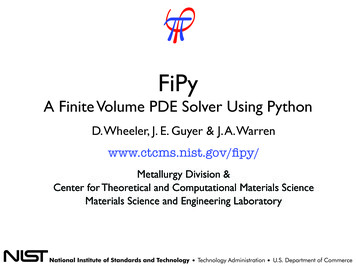
CEAC Examplespecimens (θ 0.44 and 0.88) ratherthan the predicted seams. Such depletion effects have been fully ions—Deposition in vias, unliketrenches, is a three-dimensional problem by virtue of the nonzero curvatureof the cylindrical sidewalls. Cross sections detailing the filling of cylindricalvias with a 4.5 sidewall slope areshown in 10 s increments in Fig. 7.16 Inthis experiment the catalyst is adsorbedsimultaneously with copper plating inaccord with conventional practice.Wafer fragments were immersed in theSPS-PEG-Cl electrolyte, containing 6.4µmol/L SPS, with a -0.25 V (Cu/Cu2 )growth potential already applied.Growth is essentially conformal for thefirst 60 s followed by the onset of bottom-up superfilling at 70 s. The fillingprocess is summarized by tracking theheight of the deposit along the centerline of the via, as a function of deposition time. Favorable agreement withthe CEAC simulation is evident and thecorrespondingsimulated growth conLEVELERtoursaregiveninthe inset.16ACCELERATOR#CurvatureCopper electodeposition in submicron featureselectrolyte additives influence deposition rateCEAC - Curvature Enhanced Accelerator Coverage.“Momentum plating”e of images of direct copper deposition on trenches coatedare considered only across the hydrodynamic boundary in these simulations.However, for the higher deposition ratesassociated with higher catalyst cover“Bottom Up” fillages, significant depletion of the Cu2 ion occurs within the trench, resultingin faster deposition toward the top of thefeature. This leads to an earlier impingement at this location and void formation as observed in two experimental2004 1/2coverageK Accelerator k exp αθadθa κ %v θa ka (θa0 θa )dtInterface speedfixed point movingθs withθs0 theat t 0interfaceExperimental sequenceθa θa0 at t 0θs0K0 1 K0INHIBITORSeedless Superfill45 degreeCurrentmetallizationside walltilttechnologyemploys three layers, a barrier metal,51!#K0 k exp α θa0! 1/2 "αF ϕϕπ"
! Jvθ i (k0 !k3 η 3 )cΩiθ (1" θ) ci! b!θ) m"expΩ tcm αFvi (b"1iΩcv (b0 b1 θ) expηcm 0 αFc Ω αFm nFm(b! exp "η η b1 θ)(b0 RT b1expθ)nF v c 0v c RT RTm φ Ω nF m nFcim φ αFm vcextv (b0 η φb1 θ) texp vcext φ nFRTm θ3 i t φ θ φ t Jvθ (k0 k3 η )cθ (1i0 φ 0 vext mk vθ cext φ Jvθ c θ (1 θ) t t t · Dm cm φ t c θ θ mi · Dv cext 0i φ mθ cm Jvθ k θ tcJvθ(1 θ) 0 kc(1 0θ θ · Dθ)θ tθ cθ t t cθ t θ ·Dθ cθi cm Jvθ c t m kc 0 θ) 0θθ (1 ·D c ·Dmmm cm 0v t t tDn̂· c on φ 0 cmmΩv cθ Dm n̂ c cθ ·Dmmφ · c 00 0(1 θ) om t m· D 0·on θ θ cDΩ cθ cθ·n̂Dθ θ kcθ t tDθθn̂ · cθ kθ cθ Γ(1 θ) on φ 0 c · Dθ cθ 0 t φ 1v2Dm n̂ · cm on φ 02Ωv vDθ n̂ ·D c kθ)ononn̂· c θ Γ(1φ θ mDmθ c onφ 0 φ 0 0m n̂ · cm ΩΩDθ Dn̂ · n̂ c θ)φ φ 0 0θ kθ cθ Γ(1· c kc Γ(1 θ)on onCEAC Exampleafter D. Josell, D. Wheeler, W. H. Huber, and T. P. Moffat,Physical Review Letters, 87(1), (2001) 016102# create a mesh# create the field variables# create the governing equations# create the boundary conditions# solveθθθ θ22 2ϕϕπ
! Jvθ i (k0 !k3 η 3 )cΩiθ (1" θ) ci! b!θ) m"expΩ tcm αFvi (b"1iΩcv (b0 b1 θ) expηcm 0 αFc Ω αFm nFm(b! exp "η η b1 θ)(b0 RT b1expθ)nF v c 0v c RT RTm φ Ω nF m nFcim φ αFm vcextafter D. Josell, D. Wheeler, W. H. Huber, and T. P. Moffat,v (b0 η φb1 θ) texp v φ nFcRTextPhysical Review Letters, 87(1), (2001) 016102m θ3 i t φ θ φ t Jvθ (k0 k3 η )cθ (1i0 φ 0 vext mk vθ cext φ Jvθ c θ (1 θ) t t t · Dm cm# create a mesh φ t c θ θ mi · Dv cext 0i φ mθ cmfrom gapFillMesh import TrenchMesh Jvθ k θ tcJvθ(1 θ) 0 kc(1 0θ θ · Dθ)θ tθ cθ t tmesh TrenchMesh(cellSize 0.002e-6, t cθ θ ·Dθ cθi cm JvθtrenchSpacing 1e-6, c t m kc 0 θ) 0θθ (1 ·D c ·Dmmm cm 0trenchDepth 0.5e-6,v t t tDn̂· c on φ 0 cmmboundaryLayerDepth 50e-6,Ωv cθ Dm n̂ c cθ ·Dmmφ · c 00 0(1 θ) om t m· D 0·on θ aspectRatio 2.)θ cDΩ cθ cθ·n̂Dθ θ kcθ t tDθθn̂ · cθ kθ cθ Γ(1 θ) on φ 0 c# create the field variables · Dθ cθ 0 t φ 1# create the governing equationsv2Dm n̂ · cm on φ 02# create the boundary conditionsΩv vDθ n̂ ·D c kθ)ononn̂· c θ Γ(1φ θ mDmθ c# solve onφ 0 φ 0 0m n̂ · cm ΩΩDθ Dn̂ · n̂ c θ)φ φ 0 0θ kθ cθ Γ(1· c kc Γ(1 θ)on onCEAC Exampleθθθ θ22 2ϕϕπ
! Jvθ i (k0 !k3 η 3 )cΩiθ (1" θ) ci! b!θ) m"expΩ tcm αFvi (b"1iΩcv (b0 b1 θ) expηcm 0 αFc Ω αFm nFm(b! exp "η η b1 θ)(b0 RT b1expθ)nF v c 0v c RT RTm φ Ω nF m nFcim φ αFm vcextafter D. Josell, D. Wheeler, W. H. Huber, and T. P. Moffat,v (b0 η φb1 θ) texp v φ nFcRTextPhysical Review Letters, 87(1), (2001) 016102m θ3 i t φ θ φ t Jvθ (k0 k3 η )cθ (1i0 φ 0 vext mk vθ cext φ Jvθ c θ (1 θ) t t t · Dm cm# create a mesh φ t c θ θ mi · Dv cext 0i φ mθ cm Jvθ kc(1 θ) 0 Jvθ kc(1 0 tθθ θ · Dθ)θ t# create the field variablesθ cθ t t cθ t θ ·Dθ cθi cm Jvθ c t m kc 0 θ) 0# distance variableθθ (1 ·D c ·Dmm tm cm 0v t tDn̂· c on φ 0# surface accelerator concentration cmmΩv cθ Dm n̂ c c0θ ·Dmmφ · c θ on 0 kcm· Dm c 0 ·D c 0θ (1 θ) oθDn̂· c tθθθθΩ# bulk accelerator concentration t tDθθn̂ · cθ kθ cθ Γ(1 θ) on φ 0 c · Dθ cθ 0# metal ion concentration t φ 1# interfacial velocityv2Dm n̂ · cm on φ 02ΩexchangeCurrentDensity constantCurrentDensity\vv onDθ n̂ ·D c kcΓ(1θ)ononn̂· acceleratorVar.getInterfaceVar() c φ acceleratorDependenceCurrentDensityθ* θθmDm φ 0 φ 0 0m n̂ · cm ΩΩDθ Dn̂· n̂ c θ)φ φ 0 0θ kθ cθ Γ(1currentDensity exchangeCurrentDensity* metalVar· c / bulkMetalConcentration kc Γ(1 θ)on onCEAC Exampleθθθ θ* Numeric.exp(-transferCoefficient * faradaysConstant * overpotential \/ gasConstant / temperature)2depositionRateVariable currentDensity * atomicVolume /2charge/ faradaysC2# create the governing equations# create an iteratorϕϕπ
! Jvθ i (k0 !k3 η 3 )cΩiθ (1" θ) ci! b!θ) m"expΩ tcm αFvi (b"1iΩcv (b0 b1 θ) expηcm 0 αFc Ω αFm nFm(b! exp "η η b1 θ)(b0 RT b1expθ)nF v c 0v c RT RTm φ Ω nF m nFcim φ αFm vcextafter D. Josell, D. Whe
FiPy is a computer program written in Python to solve partial differential equations (PDEs) using the Finite Volume method Python is a powerful object oriented scripting language with tools for numerics The Finite Volume method is a way to solve a set of PDEs, similar to the Finite Element or Finite Difference methods! "! "