Transcription
Tolerance Stack Analysis MethodsA Critical ReviewFritz Scholz Research and TechnologyBoeing Information & Support ServicesNovember 1995AbstractThis document reviews various ways of performing tolerance stackanalyses. This review is limited to assembly criteria which are linearor approximately linear functions of the relevant part dimensions. Beginning with the two extreme cornerstones, namely the arithmetic orworst case tolerance stack and the statistical or RSS tolerance stackmethod, various compromises or unifying paradigms are presentedwith their underlying assumptions and rationales. These cover distributions more dispersed than the commonly assumed normal distribution and shifts in the means. Both worst case and statistical stackingof mean shifts are discussed. The latter, in the form presented here,appears to be new. The appropriate methods for assessing nonassembly risk are indicated in each case. P.O. Box 3707, MS 7L-22, Seattle WA 98124-2207,e-mail: fritz.scholz@grace.rt.cs.boeing.com
Contents1 Introduction and Overview32 Notation and Conventions43 Arithmetic Tolerance Stack (Worst Case)74 Statistical Tolerancing (RSS Method)94.1Statistical Tolerancing With Normal Variation . . . . . . . . .4.2Statistical Tolerancing Using the CLT . . . . . . . . . . . . . . 144.3Risk Assessment with Statistical Tolerance Stacking . . . . . . 185 Mean Shifts9205.1Arithmetic Stacking of Mean Shifts . . . . . . . . . . . . . . . 245.2Risk Assessment with Arithmetically Stacked Mean Shifts . . 315.3Statistical Stacking of Mean Shifts . . . . . . . . . . . . . . . 345.4Statistical Stacking of Mean Shifts Revisited . . . . . . . . . . 402
1Introduction and OverviewTolerance stacking analysis methods are described in various texts and papers, see for example Gilson (1951), Mansoor (1963), Fortini (1967), Evans(1975), Cox (1986), Greenwood and Chase (1987), Kirschling (1988), Bjørke(1989), Henzold (1995), and Nigam and Turner (1995). Unfortunately, thenotation is often not standard and not uniform, making the understandingof the material at times difficult.Invariably the discussion includes the two cornerstones, arithmetic andstatistical tolerancing. This examination is no exception, since these twomethods provide conservative and optimistic benchmarks, respectively. Inthe basic statistical tolerancing scheme it is assumed that part dimensionvary randomly according to a normal distribution, centered at the toleranceinterval midpoint and with its 3σ spread covering the tolerance interval.For given part dimension tolerances this kind of analysis typically leads tomuch tighter assembly tolerances, or for given assembly tolerance it requiresconsiderably less stringent part dimension tolerances.Since practice has shown that the results are usually not quite as good asadvertised, one has tried to relax the above distributional assumptions in avariety of ways. One way is to allow other than normal distributions whichessentially cover the tolerance interval with a wider spread, but which arestill centered on the tolerance interval midpoint. This results in somewhatless optimistic gains than those obtained under the normality assumptions,but usually still much better than those given by arithmetic tolerancing,especially for longer tolerance chains.Another relaxation concerns the centering of the distribution on the tolerance interval midpoint. The realization that it is difficult to center anyprocess exactly where one wants it to be has led to several mean shift models in which the distribution may be centered anywhere within a certainneighborhood around the tolerance interval midpoint, but usually it is stillassumed that the distribution is normal and its 3σ spread is still withinthe tolerance limits. This means that while we allow some shift in the meanwe require a simultaneous reduction in variability. The mean shifts are thenstacked in worst case fashion. The correspondingly reduced variation of theshifted distributions is stacked statistically. The overall assembly tolerancethen becomes (in worst case fashion) a sum of two parts, consisting of anarithmetically stacked mean shift contribution and a term reflecting the sta3
tistically stacked distributions describing the parts variation. It turns outthat our corner stones of arithmetic and statistical tolerancing are subpartsof this more general model, which has been claimed to unify matters.However, there is another way of dealing with mean shifts which appearsto be new, at least in the form presented here. It takes advantage of statistical stacking of mean shifts and stacking that in worst case fashion with thestatistical stacking of the reduced variation in the part dimension distributions. A precursor to this can be found in Desmond’s discussion of Mansoor’s(1963) paper. However, there it was pointed out that it leads to optimisticresults. The reason for this was a flaw in handling the reduction of the partdimension variation caused by the random mean shifts.When dealing with tolerance stacking under mean shifts one has to takespecial care in assessing the risk of nonassembly. Typically only one tail ofthe assembly stack distribution is significant when operating at one of thetwo worst possible assembly mean shifts. For this reason the method of riskcalculations are discussed in detail, where appropriate.2Notation and ConventionsThe tolerance stacking problem arises because of the inability to produceparts exactly according to nominal. Thus there is the possibility that theassembly of such interacting parts will not function or won’t come togetheras planned. This can usually be judged by one or more assembly criteria,say A1 , A2 , . . .Here we will be concerned with just one such assembly criterion, say A,which can be viewed as a function of the part dimensions X1 , . . . , Xn , i.e.,A f (X1 , . . . , Xn ) .Here n may be the number of parts involved in the assembly, but n mayalso be larger than that, namely when some parts contribute more than onedimension to the assembly criterion A. Ideally the part dimensions shouldbe equal to their respective nominal values ν1 , . . . , νn . Recognizing the inevitability of part variation from nominal one allows the part dimension Xi tovary over an interval around νi . Typically one specifies an interval symmetricaround the nominal value, i.e., Ii [νi Ti , νi Ti ]. However, asymmetrictolerance intervals do occur and in the most extreme form they become unilateral tolerance intervals, e.g., Ii [νi Ti , νi ] or Ii [νi , νi Ti ]. Most4
generally one would specify a tolerance interval Ii [ci , di ] with ci νi di .When dealing with a symmetric or unilateral tolerance interval one callsthe value Ti the tolerance. For the most general bilateral tolerance interval, Ii [ci , di ], one would have two tolerances, namely T1i νi ci andT2i di νi . Although asymmetrical tolerance intervals occur in practice,they are usually not discussed much in the literature. The tolerance stackingprinciples apply in the asymmetric case as well but the analysis and exposition tends to get messy. We will thus focus our review on the symmetriccase.Sometimes one also finds the term tolerance range which refers to thefull length of the tolerance interval, i.e., Ti0 di ci . When reading theliterature or using any kind of tolerance analysis one should always be clearon the usage of the term tolerance.The function f that shows how A relates to X1 , . . . , Xn is assumed to besmooth, i.e., for small perturbations Xi νi of Xi from nominal νi we assumethat f (X1 , . . . , Xn ) is approximately linear in those perturbations, i.e.,A f (X1 , . . . , Xn ) f (ν1 , . . . , νn ) a1 (X1 ν1 ) . . . an (Xn νn ) ,where ai f (ν1 , . . . , νn )/ νi . Here one would usually treat νA f (ν1 , . . . , νn )as the desired nominal assembly dimension.Often f (X1 , . . . , Xn ) is naturally linear, namelyA f (X1 , . . . , Xn ) a0 a1 X1 . . . an Xnwith known coefficients a1 , . . . , an . The corresponding nominal assembly dimension is thenνA a0 a1 ν1 . . . an νn .Note that we can match this linear representation with the previous approximation by identifyinga0 f (ν1 , . . . , νn ) a1 ν1 . . . an νn .In the simplest form the ai coefficients are all equal to one, i.e.,A X1 . . . Xn ,or are all of the form ai 1. This occurs naturally in tolerance path chains,where dimensions are measured off positively in one direction and negatively5
in the opposite direction. In that case we would haveA X1 . . . Xn .We will assume from now on that A is of the formA a0 a1 X1 . . . an Xnwith known coefficients a0 , a1 , . . . , an . For the tolerance analysis treatmentusing quadratic approximations to f we refer to Cox (1986). Although thisapproach is more refined and appropriate for stronger curvature over thevariation ranges of the Xi , it also is more complex and not routine. It alsohas not yet gone far in accommodating mean shifts. This part of the theorywill not be covered here.We note here that not all functions f are naturally smooth. A very simplenonsmooth function f is given by the following:f (X1 , X2 ) qX12 X22which can be viewed as the distance of a hole center from the nominal origin(0, 0). This function does not have derivatives at (0, 0), its graph in 3-spacelooks like an upside cone with its tip at (0, 0, 0). There can be no tangentplane at the tip of that cone and thus no linearization. Although we havefound these kinds of problems appear in practice when performing toleranceanalyses in the context of hole center matching and also in hinge toleranceanalysis (Altschul and Scholz, 1994) there seems to be little recognition inthe literature of such situations.Let us return again to our assumption of a linear assembly criterion. Thewhole point of a tolerance stack analyses is to find out to what extent theassembly dimension A will differ from the nominal value νA while the Xiare restricted to vary over Ii . This forward analysis can then be turnedaround to solve the dual problem. For that problem we specify the amountof variation that can be tolerated for A and the task is that of specifying thepart dimension tolerances, Ti , so that desired assembly tolerance for A willbe met.Although this is a review paper, it is far from complete, as should be clearfrom the above remarks. Nevertheless, it seems to be the most comprehensivereview of the subject matter that we are aware of. Many open questionsremain.6
3Arithmetic Tolerance Stack (Worst Case)This type of analysis assumes that all part dimensions Xi are limited to Ii .One then analyzes what range of variation can be induced in A by varyingall n part dimensions X1 , . . . , Xn independently (in the nonstatistical sense)over the respective tolerance intervals. Clearly, the largest value ofA a0 a1 X1 . . . an Xn a0 a1 ν1 . . . an νn a1 (X1 ν1 ) . . . an (Xn νn ) νA a1 (X1 ν1 ) . . . an (Xn νn )is realized by taking the largest (smallest) value of Xi Ii [ci , di ] wheneverai 0 (ai 0). For example, if a1 0, then the term a1 (X1 ν1 ) becomeslargest positive when we take X1 ν1 and thus at the lower endpoint ci ofIi . Thus the maximum possible value of A isAmax max {A : Xi Ii , i 1, . . . , n} νA X(di νi )ai X(ci νi )ai .ai 0ai 0In similar fashion one obtains the minimum value of A asAmin min {A : Xi Ii , i 1, . . . , n} νA X(di νi )ai ai 0X(ci νi )ai .ai 0If the tolerance intervals Ii are symmetric around the nominal νi , i.e.,Ii [νi Ti , νi Ti ] or di νi Ti and ci νi Ti , we findAmax νA Xai Ti Xai 0ai 0XXai Ti νA ai Ti ai 0ai Ti νA ai 0 ai Tii 1andAmin νA nXnX ai Ti .i 1Thus"A [Amin , Amax ] νA nXi 1 h ai Ti , νA nXi 1νA TAarith , νA TAarith7i# ai Ti
whereTAarith nX ai Ti(1)i 1is the symmetric assembly tolerance stack. Aside from the coefficients ai ,which often are one anyway, (1) is a straight sum of the Ti ’s, whence thename arithmetic tolerance stacking.The calculated value TAarith should then be compared against QA , therequirement for successful assembly. If all part dimensions satisfy their individual tolerance requirements, i.e., Xi Ii , and if TAarith computed from (1)satisfies TAarith QA , then every assembly involving these parts will fit withmathematical certainty. This is the main strength of this type of tolerancecalculation.In the special case where ai 1 and Ti T for i 1, . . . , n we get n T , i.e., the assembly tolerance grows linearly with the number n ofpart dimensions. If proper assembly requires that TAarith QA .00400 , thenthe common part tolerances have to be T TAarith /n .00400 /n. For largen this can result in overly tight part tolerance requirements, which often arenot economical. This is the main detracting feature of this form of tolerancestack analysis. It results from the overly conservative approach of stackingthe worst case deviations from nominal for all parts. In reality, such worstcase stackup should be extremely rare and usually occurs only when it isrealized deliberately.TAarithThe assumption that all parts satisfy their respective tolerance requirements, Xi Ii , should not be neglected. Without this there is no 100%guarantee of assembly. In effect this assumption requires an inspection ofall parts, typically through simple check gauges. This form of inspection isa lot simpler than that required for statistical tolerancing. For the latterthe part measurements Xi themselves are required, at least for samples, inorder to demonstrate process stability. Samples of part measurements aremore easily amenable to extrapolation and inference about the behavior ofthe whole population. For samples of go/no-go data this would be a lot moredifficult. There may be a cost tradeoff here, namely 100% part checking byinexpensive gauging versus part sampling (less than 100%) with expensivemeasuring.Another plus for the arithmetic tolerancing scheme is that the underlyingassumptions are very minimal, as can be more appreciated in the next section.8
4Statistical Tolerancing (RSS Method)The previous section employed a form of tolerance stacking that guardsagainst all allowed variation contingencies by stacking the part tolerances inthe worst possible way. It was pointed out that this can only happen whendone deliberately, i.e., choosing the worst possible parts for an assembly.If one were to choose parts in a random fashion, such a worst case assemblywould be extremely unlikely. Typically the part deviations from nominal willtend to average out to some extent and the tolerance stack should not be asextreme as portrayed under the arithmetic tolerance stacking scheme. Statistical tolerancing exploits this type of variation cancellation in a systematicfashion.We will introduce the method under a certain standard set of assumptions, first assuming a normal distribution describing the part variation, thenrelaxing this to other distributions by appealing to the central limit theorem(CLT), and we finally address the issue of assessing the risk of nonassembly.4.1Statistical Tolerancing With Normal VariationThe following standard assumptions are often made when first introducingthe method of statistical tolerancing. These should not necessarily be accepted at face value. More realistic adaptations will be examined in subsequent sections.Randomness: Rather than assuming that the Xi can fall anywhere in thetolerance interval Ii , even to the point that someone maliciously anddeliberately selects parts for worst case assemblies, we assume here thatthe Xi vary randomly according to some distributions with densitiesfi (x), i 1, . . . , n, and cumulative distribution functionsFi (t) Ztf (x) dx ,i 1, . . . , n. The idea is that most of the occurrences of Xi will fall inside Ii , i.e.,most of the area under the density fi (x) falls between the endpoints ofIi . As a departure from worst case tolerancing we do accept a certainsmall fraction of part dimensions that will fall outside Ii . This freesus from having to inspect every part dimension for compliance with9
the tolerance interval Ii . Instead we ask/assume that the processesproducing the part dimensions are stable (in statistical control) andthat these part dimensions fall mostly within the tolerance limits. Thisis ascertained by sampling only a certain portion of parts and measuringthe respective Xi ’s.Independence: The independence assumption is probably the most essential corner stone of statistical tolerancing. It allows for some cancellation of variation from nominal.Treating the Xi as random variables, we also demand that these randomvariables are (statistically) independent. This roughly means that thedeviation Xi νi has nothing to do with the deviation Xj νj fori 6 j. In particular, the deviations will not be predominantly positiveor predominantly negative. Under independence we expect to get amixed bag of negative and positive deviations which essentially allowsfor some variation cancellation. Randomness alone does not guaranteesuch cancellation, especially not when all part dimension show randomvariation in the same direction. This latter phenomenon is exactlywhat the independence assumption intends to exclude.Typically the independence assumption is reasonable when part dimensions pertain to different manufacturing/machining processes. However, situations can arise where this assumption is questionable. Forexample, several similar/same parts (coming from the same process)could be used in the same assembly. Thermal expansion also tends toaffect different parts similarly.Distribution: It would be nice to have data on the part dimension variation, but typically that is lacking at the design stage. For that reasonone often assumes that fi is a normal or Gaussian density over the interval Ii . Since that latter is a finite interval and the Gaussian densityextends over the whole real line R ( , ), one needs to strike acompromise. It consists in asking that the area under the density fiover the interval Ii should represent most of the total area under fi ,i.e.Zfi (x) dx 1 .Ii10
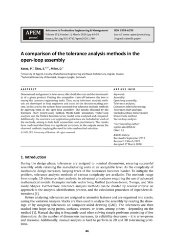
Figure 1: Normal Distribution Over Tolerance Intervalλ i-T iλi11λ i Ti
In fact, most proposals ask forZIifi (x) dx .9973 .This rather odd looking probability ( 1) results from choosing fi tobe a Gaussian density with mean µi νi at the center of the toleranceinterval and with standard deviation σi Ti /3, i.e.,x µi1ϕσiσi fi (x) 12where ϕ(x) e x /22π ,is the standard normal density. We thus haveIi [νi Ti , νi Ti ] [µi 3σi , µi 3σi ]andZIifi (x) dx µi 3σiZµi 3σiZ1x µiϕσiσi dx3ϕ(x) dx Φ(3) Φ( 3) .9973 , 3whereΦ(t) Ztϕ(x) dx is the standard normal cumulative distribution function.Thus the odd looking probability .9973 is the result of three assumptions, namely i) a Gaussian density fi , ii) νi µi , i.e., the part dimension process is centered on the nominal value, and iii) Ti 3σi . Thefirst two assumptions make it possible that the simple and round factor 3 in 3σi produces the probability .9973. This is a widely acceptedchoice although others are possible. For example, Mansoor (1963) appears to prefer the factor 3.09 resulting in a probability of .999 for partdimension tolerance compliance.One reason that is often advanced for assuming a normal distribution isthat the deviations from nominal are often the result of many additivecontributors which are random in nature, and each of relatively smalleffect. The central limit theorem (see next section) is then used to claim12
normality for the sum of many such contributors. It is assumed thatthe person producing the part will aim for the nominal part dimension,but for various reasons there will be deviations from the nominal whichaccumulate to an overall deviation from nominal, which then is claimedto be normal. Thus the values Xi will typically cluster more frequentlyaround the nominal νi and will less often result in values far away. Thisview of the distribution of Xi represents an important corner stone inthe method of statistical tolerancing.Under the above assumptions we can treat the assembly criterionA a0 a1 X1 . . . an Xnas a random variable, in fact as Gaussian random variable with meanµA a0 a1 µ1 . . . an µn a0 a1 ν1 . . . an νn νAand with variance2 1 2 2T122 Tn2 2 . a aT . aT.n11nn323232The first equation states that the mean µA of A coincides with the nominalvalue νA of A. This results from the linear dependence of A on the part dimensions Xi and from the fact that the means of all part dimensions coincidewith their respective nominals. The above formula for the variance can berewritten as followsσA2 a21 σ12 . . . a2n σn2 a213σA qa21 T12 . . . a2n Tn2 .If we call 3σA TARSS , we get the well known RSS-formula for statisticaltolerance stacking:qRSS(2)TA a21 T12 . . . a2n Tn2 .Here RSS refers to the root/sum/square operation that has to be performedto calculate TARSS . Since A is Gaussian, we can count on 99.73% of all assembly criterion values A to fall within 3σA TARSS of its nominal νA , oronly .27% of all assemblies will fail.What have we gained for the price of tolerating a small fraction of assembly failures? Again the answer becomes most transparent when all parttolerance contributions ai Ti are the same, i.e., ai Ti T . Then we have TARSS T n13
as opposed to T arith T n in arithmetic tolerancing. The factor n growsa lot slower than n. Even for n 2 we find that 2 1.41 is 29% smallerthan 2 and for n 4 we have that 4 is 50% smaller than 4.00If proper assembly requires that TARSS QA .004 , then the commonRSSpart tolerance contributions have to be T TA / n .00400 / n. Dueto the divisor n, these part tolerances are much more liberal than thoseobtained under arithmetic tolerancing.4.2Statistical Tolerancing Using the CLTOne assumption used heavily in the previous section is that of a Gaussiandistribution for all part dimensions Xi . This assumption has often been challenged, partly based on part data that contradict the normality, partly basedon mean shifts that result in an overall mixture of normal distributions, i.e.,more smeared out, and last but not least based on the experience that theassembly fallout rate was higher than predicted by statistical tolerancing.We will here relax the normality assumption by allowing more general distributions for the part variations Xi . However, we will insist that the meanµi of Xi still coincides with the nominal νi . Relaxing this last constraint willbe discussed in subsequent sections.To relax the normality assumption for the part dimensions Xi we appealto the central limit theorem of probability theory (CLT). In fact, we will nowuse the following assumptions1. The Xi , i 1, . . . , n, are statistically independent.2. The density fi governing the distribution of Xi has mean µi νi andstandard deviation σi .3. The variability contributions of all terms in the linear combination Abecome negligible for large n, i.e.,max (a21 σ12 , . . . , a2n σn2 ) 0 as n .a21 σ12 . . . a2n σn2Under these three conditions1 the Lindeberg-Feller CLT states that the linear1In fact, they need to be slightly stronger by invoking the more technical Lindebergcondition, see Feller (1966).14
combinationA a0 a1 X1 . . . an Xnhas an approximately normal distribution with meanµA a0 a1 µ1 . . . an µn a0 a1 ν1 . . . an νn νAand with varianceσA2 a21 σ12 . . . a2n σn2 .Assumption 3 eliminates situations where a small number of terms in thelinear combination have so much variation that they completely swamp thevariation of the remaining terms. If these few dominating terms have nonnormal distributions, it can hardly be expected that the linear combinationhas an approximately normal distribution.In spite of the relaxed distributional assumptions for the part dimensions we have that the assembly criterion A is again approximately normallydistributed and its mean µA coincides with the desired nominal value νA(because we deal with a linear combination and since we assumed µi νi ).From the approximate normality of A we can count on about 99.73% of allassembly criteria to fall within [νA 3σA , νA 3σA ].This is almost the same result as before, except for one “minor” point.In the previous section we had assumed a particular relation between thepart dimension σi and the tolerance Ti , namely we stipulated that Ti 3σi .This was motivated mainly by the fact that under the normality assumptionalmost all (99.73%) part dimensions would fall within 3σi of the nominalνi µi . Without the normality assumption for the parts there is no suchhigh probability assurance for such 3σi ranges. However, the Camp-Meidellinequality (Encyclopedia of Statistical Sciences, Vol. I, 1982), states that forsymmetric and unimodal densities fi with finite variance σi2 we haveP ( Xi µi 3σi ) 1 4 .9506.81Here symmetry means that fi (νi y) fi (νi y) for all y, and thus thatµi νi . Unimodality means that fi (νi y) fi (νi y 0 ) for all 0 y y 0 ,i.e., the density falls off as we move away from its center, or at least it doesnot increase. Although this covers a wide family of reasonable distributions,the number .9506 does not carry with it the same degree of certainty as .9973.15
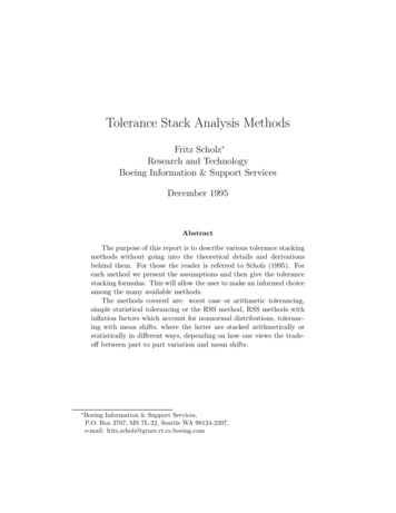
We thus do not yet have a natural link between the standard deviationσi and the part dimension tolerance Ti . If the distribution of Xi has a finiterange, then one could equate that finite range with the Ti tolerance rangearound νi . This is what has commonly been done. In the case of a Gaussianfi this was not possible (because of the infinite range) and that was resolvedby opting for the 3σi Ti range. By matching the finite range of adistribution with the tolerance range [νi Ti , νi Ti ] we obtain the linkbetween σi and Ti , and thus ultimately the link between TA and Ti . Since thespread 2Ti of a such finite range distribution can be manipulated by a simplescale change which also affects the standard deviation of the distribution bythe same factor it follows that σi and Ti will be proportional to each other,i.e., we can stipulate thatcTi 3σi ,where c is a factor that is specific to the type of distribution. The choice oflinking this proportionality back to 3σi facilitates the comparison with thenormal distribution, for which we would have c cN 1.Assuming that the type of distribution (but not necessarily its locationand scale) is the same for all part dimensions we getTARSS,c 3σA q q(3a1 σ1 )2 . . . (3an σn )2(ca1 T1 )2 . . . (can Tn )2 cqa21 T12 . . . a2n Tn2 c TARSS .This leads to tolerance stacking formulas that essentially agree with (2),except that an inflation factor, c, has been added. If the distribution type alsochanges from part to part (hopefully with good justification), i.e., we havedifferent factors c1 , . . . , cn , we need to use the following more complicatedtolerance stacking formula:TARSS,c q(c1 a1 T1 )2 . . . (cn an Tn )2 ,(3)where c (c1 , . . . , cn ).In Table 1 we give a few factors that have been considered in the literature,see Gilson (1951), Mansoor (1963), Fortini (1967), Kirschling (1988), Bjørke(1989), and Henzold (1995). The corresponding distributions are illustrated16
Figure 2: Tolerance Interval Distributions & Factorsc 1c 1.732normal densityuniform densityc 1.225c 1.369triangular densitytrapezoidal density: a .5c 1.5c 1.306elliptical densityhalf cosine wave densityc 2.023c 1.134beta density: a .6, b .6beta density: a 3, b 3c 1.342c 1.512DIN - histogram density: p .7, f .4beta density: a 2, b 2 (parabolic)17
Table 1: Distributional Inflation alqcosine half wave1.306elliptical1.53(1 a2 )/2 3/ 2a 1beta (symmetric) q3 (1 p)(1 f ) f 2histogram density (DIN)in Figure 2. For a derivation of these factors see Appendix A. For the betadensity the parameters a 0 and b 0 are the usual shape parameters, a inthe trapezoidal density indicates the break point from the flat to the slopedpart of the density, and p and f characterize the histogram density (see thelast density in Figure 2), namely the middle bar of that density covers themiddle portion νi f Ti of the tolerance interval and its area comprises 100p%of the total density.Some factors have little explicit justification and motivation and are presented without proper reference. For example, the factor c 1.6 of Gilson(1951) derives from his crucial empirical formula (2) which is prefaced by“Without going deeply into a mathematical analysis . . .” Evans (1975) seemsto welcome such lack of mathematical detail by saying: “None of the resultsare derived, in the specialized sense of this word, so that it is readable byvirtually anyone who would be interested in the tolerancing problem.”Bender (1962) gives the factor 1.5 based mainly on the fact that production operators will usually give you 2/3 of the true spread ( 3σ range undera normal distribution) when asked what tolerance limits they can hold and“quality control people recognize that this 2/3 total spread includes about95% of the pieces.” To make up for these optimistically stated tolerances,Bender suggests the factor 3/2 1.5.4.3Risk Assessment with Statistical Tolerance StackingIn this section we discuss the assembly risk, i.e., the chance that an assemblycriterion A will not satisfy its requirement. As in the previous section it isassumed that all part dimensions Xi have symmetric distributions centered18
on their nominals, i.e., with means µi νi , and variances σi2 , respectively.The requirement for successful assembly is assumed to be A νA K0 ,where K0 is some predetermined number based o
This document reviews various ways of performing tolerance stack analyses. This review is limited to assembly criteria which are linear or approximately linear functions of the relevant part dimensions. Be-ginning with the two extreme cornerstones, namely the arithmetic or worst case tolerance stack and the statistical or RSS tolerance stack