WIXLIB

ancing, especially for tolerance chains involving many detail parts.Another relaxation of assumptions concerns the centering of the distribution on the tolerance interval midpoint. The realization that it is difficult tocenter any process exactly where one wants it to be has led to several meanshift models. In these the distribution may be centered anywhere within acertain small neighborhood around the nominal tolerance interval midpoint,but usually it is still assumed that the distribution is normal and its 3σspread is within the tolerance limits. This means that while we allow someshift in the detail process mean we either require a simultaneous reduction inpart variability or we have to widen the tolerance interval. The mean shiftsare then stacked in worst case fashion. The variation of the shifted distributions is stacked statistically. The overall assembly tolerance then becomes(in worst case fashion) a sum of two parts, consisting of an arithmeticallystacked mean shift contribution and a term reflecting the statistically stackedpart variation distributions. It turns out that our cornerstones of arithmeticand statistical tolerancing are special cases of this more general model, whichhas been claimed (Greenwood and Chase, 1987) to unify matters.However, there is another way of dealing with mean shifts which appearsto be new, at least in the form presented here. It takes advantage of statisticalstacking of mean shifts and stacking that aggregate in worst case fashion withthe statistical stacking of the part variation distributions. A precursor to thiscan be found in Desmond’s discussion of Mansoor’s (1963) paper. However,there it was pointed out that it leads to optimistic results. We discuss theissues involved and present several variations on that theme.Other fixes augment the statistical tolerancing method with blanket tolerance inflation factors with more or less compelling reasons. It turns outthat one of the above mentioned mean shift treatments results in just suchan inflation factor, with the size of the factor linked explicitly to the amountof tolerated mean shift.When dealing with tolerance stacking under mean shifts one has to takespecial care in assessing the risk of nonassembly. Typically only one tail ofthe assembly stack distribution is significant when operating at one of thetwo worst possible assembly mean shifts. One can take advantage of this byreducing the assembly tolerance by some small amount. We indicate brieflyhow this is done but refer to Scholz (1995) for more details.3

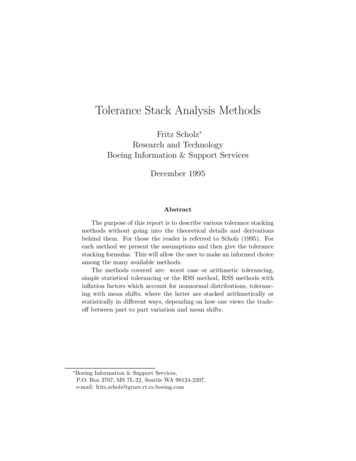
2Notation and Problem FormulationThe tolerance stacking problem arises in the context of assemblies from interchangeable parts because of the inability to produce or join parts exactlyaccording to nominal. Either the relevant part dimension varies around somenominal value from part to part or it is the act of assembly that leads to variation.For example, as two parts are joined via matching hole pairs there is notonly variation in the location of the holes relative to nominal centers on theparts but also the slippage variation of matching holes relative to each otherwhen fastened.Thus there is the possibility that the assembly of such interacting partswill not function or won’t come together as planned. This can usually bejudged by one or more assembly criteria, say G1 , G2 , . . .Here we will be concerned with just one such assembly criterion, say G,which can be viewed as a function of the part dimensions L1 , . . . , Ln . Asimple example is illustrated in Figure 1, where n 6 andG L1 (L2 L3 L4 L5 L6 ) L1 L2 L3 L4 L5 L6(1)is the clearance gap of interest. It determines whether the stack of cogwheelswill fit within the case or not. Thus it is desired to have G 0, but forfunctional performance reasons one may also want to limit G from above.A graphical representation of equation (1) is given in Figure 2, where thevarious dimensions L1 , L6 , L5 , L4 , L3 , and L2 are represented by vectorschained together, L1 butting into L6 , L6 butting into L5 (after changingdirection), L5 butting into L4 , L4 butting into L3 , and L3 butting into L2 .The remaining gap to make L2 butt up to L1 is the assembly tolerance gapof interest, namely G. This type of linkage is called a tolerance path ortolerance chain. Note that the arrows point right for positive contributionsand left for negative ones.As was pointed out before, the actual lengths Li may differ from thenominal lengths λi by some amount. If there is too much variation in theLi there may well be significant problems in satisfying G 0. Thus it is4

Figure 1: Tolerance Stack ExampleL1L3L2L5L4L6GFigure 2: Tolerance Chain Graph. . . . . . . . . . . . . . GL2L1L3L45L5L6

prudent to limit these variations through tolerances. Such tolerances, Ti ,represent an “upper limit” on the absolute difference between actual andnominal values of the ith detail part dimension, i.e., Li λi Ti . It ismainly in the interpretation of this last inequality that the various methodsof tolerance stacking differ.The nominal value γ of G is usually found by replacing in equation (1)the actual Li ’s by the corresponding nominal values λi , i.e.,γ λ1 λ2 λ3 λ4 λ5 λ6 .If the objective is to achieve a gap G that is positive and not too large (forother functional reasons) then one would presumably design the assembly insuch a way that the nominal gap γ satisfies this goal, with the hope thatthe actual gap G be not too different from γ. Thus the quantity G γ is ofconsiderable interest. It can be expressed as follows in terms of i Li λi ,the detail deviations from nominal,G γ (L1 λ1 ) (L2 λ2 ) (L3 λ3 ) (L4 λ4 ) (L5 λ5 ) (L6 λ6 ) 1 2 3 4 5 6 .The main question of tolerance stacking is the bounding of the assemblyerror or assembly misfit G γ when given tolerance bounds Ti on the detailpart errors, i.e. i Li λi Ti . In the following we will present severalsuch bounds and state under what assumptions they are valid. Before doingso we generalize the above example to a generic tolerance chain and in theprocess widen the scope to smooth sensitivity analysis problems.Above we had an assembly with a stack of six parts that involved one positive and five negative contributions. This can obviously be generalized to ndetail parts with various configurations of positive and negative contributorydirections in the tolerance chain. Hence in general we have:G a1 L1 a2 L2 a3 L3 . . . an Ln ,6

Figure 3: Function BoxX1X2X3X4X5X6X7. . . . . . . . . . . . . . . . . . . . . . . . . . . . . . . . . . . . . . . . . . . . . . . . . . . . . ., . . . ,. X. . . . . . . .f (XY. . 1., X. .2 . . . . .7 ). . . Y. . . . . . . . . . . . . . . . .where the coefficients a1 , . . . , an are either 1 or 1, independently of eachother. Our introductory example had n 6 and a1 1, a2 . . . a6 1.This then leads toG γ a1 (L1 λ1 ) a2 (L2 λ2 ) . . . an (Ln λn ) a1 1 a2 2 . . . an nas the primary object of tolerance stack analysis.From here it is only a small step to extending these methods to sensitivityanalysis in general. Those not interested in this generalization can skip tothe beginning of the next section.Rather than butting parts end to end and forming an arithmetic sum of terms with some resultant output G, we can view this relation as a moregeneral input/output relation. To get away from the restrictive notion oflengths we will use X1 , . . . , Xn as our inputs (in place of L1 , . . . , Ln ) and Y(in place of the gap G) as our output. However, here we allow more generalrules of composition, namelyY f (X1 , . . . , Xn ) ,where f is some known, smooth function which converts the inputs X1 , . . . , Xninto the output Y . This is graphically depicted in Figure 3. As an example7

of such a more general relationship consider some electronic device with components (capacitors, resistances, etc.) of various types. There may be severalperformance measures for such a device and Y may be any one of them. Giventhe performance ratings X1 , . . . , Xn of the various components, physical lawsdescribe the output Y in some functional form, which typically is not linear.The design of such an electronic device is based on nominal values, ν1 , . . . , νn ,for the component ratings. However, the actual characteristics X1 , . . . , Xnwill typically be slightly different from nominal, resulting in slight deviationsfor the actual Y f (X1 , . . . , Xn ) from the nominal ν f (ν1 , . . . , νn ). Sincethese component deviations are usually small we can reduce this problem tothe previous one of mechanically stacked parts by linearizing f , namely useY f (X1 , . . . , Xn ) f (ν1 , . . . , νn ) a1 (X1 ν1 ) . . . an (Xn νn ) a0 a1 X1 . . . an Xnwhere ai f (ν1 , . . . , νn )/ νi , i 1, . . . , n anda0 f (ν1 , . . . , νn ) a1 ν1 . . . an νn .Note: for this linearization to work we have to assume that f has continuousfirst partial derivatives at (ν1 , . . . , νn ).Aside from the term a0 we have again the same type of arithmetic sumfor our “assembly” criterion Y as we had in the mechanical tolerance stack.However, here the ai are not restricted to the values 1. The additional terma0 1 does not present a problem as far as variation analysis is concerned, sinceit is constant and known.Again we like to understand how far Y may vary from the nominal ν f (ν1 , . . . , νn ). From the above we haveY ν a1 (X1 ν1 ) . . . an (Xn νn ) a1 1 . . . an n ,i.e., just as before, the only difference being that the ai are not restricted to 1. Since all the tolerance stacking formulas to be presented below will be1it is based on the nominal and known quantities ν1 , . . . , νn8

given in terms of these ai and since nowhere use was made of ai 1, itfollows that they are valid for general ai and thus for the sensitivity problem.There are situations in which a functional relation Y f (X1 , . . . , Xn ),although smooth, is not very well approximated by a linear function, at leastnot over the range of variation envisioned for the Xi . In that case one coulduse a quadratic approximation to capture any relevant curvature in f . Tolerance stacking methods using this approach are covered in Cox (1986). Thesemethods are fairly complex and still quite restrictive in the assumptions under which they are valid. Of course, it may be possible to extend thesemethods along the same lines as presented here for linear tolerance stacks.As noted above, the linearization will work only for smooth functions f .To illustrate this with a counterexample, where linearization fails completely,consider the function f (X1 , X2 ) X12 X22which can be viewed as the distance of a hole center from the nominal origin(0, 0). This function does not have derivatives at (0, 0), its graph in 3-spacelooks like an upside cone with its tip at (0, 0, 0). There can be no tangentplane at the tip of that cone and thus no linearization. Another examplewhere such linearization fails is discussed in Altschul and Scholz (1994). Itinvolves hinge mating and the problem arises due to simultaneous and thusminimum gap requirements.In presenting the tolerance stacking formulas we will return to using Liand λi for the part dimensions and nominals. Those that wish to apply theseconcepts to sensitivity analysis should have no problem replacing Li , G, λi byXi , Y, νi , respectively.3Tolerance Stacking FormulasIn this section we will present various formulas for tolerance stacking. Bytolerance stacking we mean a rule that combines the detail tolerances Tiinto an assembly tolerance Tassy . Typically Tassy is a monotone increasingfunction of the Ti . Thus, if the resulting Tassy is too large, one can counteractthat by reducing all or some of the Ti , which usually makes for costlierpart production. On the other hand, if Tassy is smaller than required forsuccessful assembly fit, then one can loosen the detail tolerances Ti , with9

some possibility of cost reduction.Why do we have more than one formula for tolerance stacking and whyso many? One reason for this is that these methods have evolved and arestill evolving, partly responding to economic pressures and partly because ofthe nature of the problem. Namely, it all depends on what assumptions oneis willing to make.Fewer assumptions entail broader applicability but one also will get lessout of a tolerance stack analysis, i.e., one will wind up with fairly wideassembly tolerance limits or, when trying to counteract that through the Ti ,with very tight and thus costly detail tolerance requirements.With more knowledge about the manufacturing processes one may feelcomfortable with more assumptions, resulting in tighter assembly tolerancelimits or, if those can be relaxed, with looser detail tolerance requirements.Thus it is very important to be aware of the assumptions behind the various methods. We will begin the presentation of stacking methods with theworst case or arithmetic method, which tends to be most conservative. Thisis followed by the conventional RSS or statistical tolerance stacking method,which tends to be on the optimistic side. This results from imposing somerather stringent assumptions. If the arithmetic stacking method gives satisfactory assembly tolerance results, then there is little motivation to try anyof the other methods, except possibly to relax detail tolerances to achievecost reduction. If the RSS method does not give satisfactory assembly tolerance results, then any of the other methods will not make matters anybetter. Then the only recourse is to tighten detail tolerances or, if that isnot feasible, change the design.After discussing these two basic and well known methods we will discussseveral hybrid tolerance stacking methods which impose assumptions whichare more likely to be met in practice. As a result the assembly tolerances liesomewhere between those corresponding to the two classical methods.10

3.1Arithmetic or Worst Case Tolerance StackingAssuming i Li λi Ti for all i 1, 2, . . . , n we can bound G γ byarithTassy a1 T1 a2 T2 . . . an Tn .(2)If ai 1 for all i, this simplifies toarithTassy T1 T2 . . . Tn .The validity hinges solely on the above assumption. Thus, no matter howthe detail dimensions Li deviate from their nominal values λi within theconstraint Li λi Ti , the difference G γ is guaranteed to be boundedarith. This guarantee is the main strength of this method. However, oneby Tassyshould not neglect to make sure that the assumptions are met, i.e., detailparts need to be inspected to see whether Li λi Ti or not.arithgrows more or less linearlyThe main weakness of the method is that Tassywith n. This is most easily seen when the detail part tolerance contributions ai Ti are all the same, i.e., ai Ti Tdetail in which casearithTassy n · Tdetail .By inverting this we getarithTassy,Tdetail nwhich tells us how to specify detail tolerances from assembly tolerances.As assemblies grow, i.e., as n gets large, these requirements on the detailtolerances can get quite severe.arithresults from assuming a devil’s advocate poThe linear growth of Tassyarith, namely by always taking the detailsition in deriving the formula for Tassypart variation in such a way as to make the assembly criterion G differ asmuch as possible from γ. This is the reason for the method’s alternate name:worst case tolerancing.If the detail tolerances are not all the same, it is more complicated toarrive at appropriate detail tolerances satisfying a given assembly tolerancerequirement. For example, suppose Ti ρi T1 for i 2, . . . , n. ThenarithTassy T1 ρ2 T1 . . . ρn T1 T1 (1 ρ2 . . . ρn )11

so thatT1 arithTassy,1 ρ2 . . . ρnandTi arithρi Tassy1 ρ2 . . . ρnarithfor i 2, . . . , n. Thus relaxing or tightening Tassyby some factor affects alldetail tolerances Ti by the same factor.One may also want to treat the detail tolerances Ti in a more differentiatedmanner, i.e., leave some as they are and reduce other significantly in order toachieve the desired assembly tolerance. This easily done in iterative fashionusing the forward formula (2).The above considerations on how to set detail tolerances based on assembly tolerance requirements can be carried out for the other types of tolerancestacking as well and we leave it up to the reader to similarly use the varioustolerance stacking formulas in reverse.3.2RSS Method or Statistical TolerancingUnder this method of tolerance stacking a very important new element isadded to the

Tolerance stack analysis methods are described in various books and pa-pers, see for example Gilson (1951), Mansoor (1963), Fortini (1967), Wade 7),Kirschling . analysis typically leads to much tighter assembly tolerances, or for given