Transcription
Upps al a U ni versity log otypeIT 22 051Degree project 30 creditsAugust 2022Geospatial TimeseriesImputation using Deep NeuralNetworksMattis KienmayerMaster’s Pr ogramme in Imag e Anal ysisand M ac hine Learni ngMaster’s Programme in Image Analysisand Machine Learning
Upps al a U ni versity log otypeGeospatial Timeseries Imputation using Deep Neural NetworksMattis KienmayerAbstractWith the advancement of technology, data collection has become a big part of many industries.Large amounts of data can be used for analytics purposes, and give companies the opportunityto offer a wider range of services to their customers. Due to the ever-increasing interest in data,and due to restrictive regulations such as the General Data Protection Regulation (GDPR),synthetic data generation is gaining attention from researchers in both industry and academia.Scania collects vehicle data from more than 450,000 trucks and buses worldwide, and use thisfor diagnostics and fleet management purposes. However, the frequency of data collection istailored to customer needs, and Scania could still benefit from having access to higher temporalresolution data.This project investigates the possibility of using deep learning methods for the purpose ofincreasing the temporal resolution in geospatial time series. Specifically, a classic feed forwardnetwork as well as a Generative Adversarial Network (GAN) is evaluated and compared to asimpler, more intuitive nearest neighbour based baseline model.While deep neural network complexity allow for reasonable quantitative results, qualitativeevaluations show that the spatial context of geospatial data is hard for the models to learn.Without any conditioning on road networks, the models generate vehicle positions that are notalways realistic.Fac ulty of Sci enc e and Technol og y, U ppsal a U ni versity. U pps ala. Super vis or: Kuo-Yun Liang, Subjec t reader: Ingela N ystr öm, Examiner: N ataš a Sladoj eFaculty of Science and TechnologyUppsala University, UppsalaSupervisor: Kuo-Yun Liang Subject reader: Ingela NyströmExaminer: Nataša Sladoje
Contents1 Introduction1.1 Background and Motivation . . . . . . . . . . . . . . . . . . . . . . . . . . . . . .1.2 The Data . . . . . . . . . . . . . . . . . . . . . . . . . . . . . . . . . . . . . . . .1.3 Problem Description & Aim . . . . . . . . . . . . . . . . . . . . . . . . . . . . . .66662 Related Work83 Theory3.1 Time Series . . . . . . . . . . . .3.2 Supervised Learning . . . . . . .3.3 Recurrent Neural Networks . . .3.4 Generative Adversarial Networks.99910114 Methods4.1 Data Pre-processing . . . . . . . . . . . . .4.1.1 Data Filtering . . . . . . . . . . . .4.1.2 Adaptive Downsampling . . . . . . .4.2 Evaluation Metrics . . . . . . . . . . . . . .4.3 Baseline Models . . . . . . . . . . . . . . . .4.3.1 A Nearest Neighbour Approach . . .4.3.2 Spatial Midpoint Road Snapping . .4.4 Main Models . . . . . . . . . . . . . . . . .4.4.1 Additional Data Processing . . . . .4.4.2 Model Design . . . . . . . . . . . . .4.4.3 Model Training and Hyperparameter. . . . . . . . . . . . . . . . . . . . . . . . . . . . . . . . . . . . . . . . .Tuning.1212121213141415151515165 Results and Discussion5.1 Vanilla Generator . . . . . .5.2 GAN . . . . . . . . . . . . .5.3 Partial GAN . . . . . . . .5.4 Nearest Neighbour Baseline5.5 Final Comparisons . . . . .1919202123246 Closing Remarks6.1 Conclusions . . . . . . . . . . . . . . . . . . . . . . . . . . . . . . . . . . . . . . .6.2 Future Work . . . . . . . . . . . . . . . . . . . . . . . . . . . . . . . . . . . . . .6.3 Acknowledgements . . . . . . . . . . . . . . . . . . . . . . . . . . . . . . . . . . .26262627.2.
List of Figures12345678910111213141516Illustration of an RNN unit. . . . . . . . . . . . . . . . . . . . . . . . . . . . . . .Illustraion of an LSTM unit. . . . . . . . . . . . . . . . . . . . . . . . . . . . . .Area coverage of data after pre-processing. . . . . . . . . . . . . . . . . . . . . . .Illustration of two subtrips where parts of the subtrips are along the same route.Illustration of the generator architecture. . . . . . . . . . . . . . . . . . . . . . .Illustration of the GAN. . . . . . . . . . . . . . . . . . . . . . . . . . . . . . . . .Vanilla generator training history. . . . . . . . . . . . . . . . . . . . . . . . . . . .Examples of upsampled sequences using the vanilla generator trained with MAEloss. Examples of subtrips upsampled using the generator. Red points are theground truth and blue points are the upsampled points. . . . . . . . . . . . . . .Example of upsampled sequence using the vanilla generator trained with MAEloss. Distance error on this sequence is DH 261. Red points are the groundtruth and blue points are the upsampled points. . . . . . . . . . . . . . . . . . . .Training history for the GAN with parameters (k1 , k2 ) (1, 3). . . . . . . . . . .Examples of upsampled sequences using the GAN, trained with (k1 , k2 ) (1, 3).Red points are the ground truth and blue points are the upsampled points. . . .Training history of the Partial GAN, using α 1/8. . . . . . . . . . . . . . . . .Examples of upsampled sequences using the PGAN, trained with α 1/8. Redpoints are the ground truth and blue points are the upsampled points. . . . . . .Examples of subtrips upsampled using the nearest neighbour approach. Redpoints are the ground truth and blue points are the upsampled points. . . . . . .A closer look at the subtrip shown in figure 14a. Red points are the ground truthand blue points are the upsampled points. To the right, we can see that thegenerated point is on the wrong lane. . . . . . . . . . . . . . . . . . . . . . . . . .Histograms of true 3 point angles (left) and 3 point angles generated by the nearestneighbour model (right). Angular values are between 0 and 180 degrees. . . . . .310111214161719202021212222232425
List of Tables123456Example of data collection spacing for subscription of 10 minute timer. . . . . . .Example of data to impute. . . . . . . . . . . . . . . . . . . . . . . . . . . . . . .Evaluation results for the vanilla generator, trained using different loss functions.Evaluation results for the GAN model, trained using different sets of parameters(k1 , k2 ). . . . . . . . . . . . . . . . . . . . . . . . . . . . . . . . . . . . . . . . . .Evaluation results for the partial GAN, trained using different values α. . . . . .Comparison of the different models performance on the test set. The JSD iscomputed using the distributions of 3 point rotations as defined by (14). . . . . .46719202224
AcronymsGAN Generative Adversarial NetworkGDPR General Data Protection RegulationJSD Jensen–Shannon DistanceLSTM Long Short-Term MemoryMAE Mean Absolute ErrorMSE Mean Squared ErrorRNN Recurrent Neural Network5
1Introduction1.1Background and MotivationScania is a leading actor in the heavy transport industry and manufactures trucks and busesfor use in many parts of the world. While logistics and cost effective transport is the main focusof the company, services such as fleet management have started taking up a larger portion of thecompany’s business. As such, data that Scania collects from its vehicles are becoming of greaterinterest, use and value. With more than 450,000 connected vehicles worldwide, the amount ofdata collected is very large and can be used for tasks such as diagnosis and logistic optimization.Even though the amount of data collected is large, there is still an interest for synthetic dataand its potential in research and development.Data is collected from Scanias vehicles at varying frequencies, depending on the customersneeds. Although the data collection is tailored specifically to suit the customer, Scania couldstill benefit from having access to higher temporal resolution data. A "simple" solution to thisproblem could be to offer customers more data collection as a standard, however this comes withadditional costs. For these reasons, Scania would like to explore the possibility of using neuralnetworks for increasing the temporal resolution on spatio-temporal data.1.2The DataThe data set used in this project comes from Scania’s Fleet Management. It consists of datacollected from Scania trucks and buses in Sweden starting from January 2019 until September2020. The data contains information including Truck/bus ID Geographical position Timestamp Ignition status Trigger type OdometerAs the fifth item suggests, data collection is event based. Data collection is triggered whenpre-determined events such as an ignition change occur. One such event is a timer; If thetimer runs out, data collection is triggered. As such, there is an upper limit on how much timecan be between two data points. This timer is what is set differently depending on customersubscriptions, i.e. one customer could have trucks with timers set to one minute, while a differentcustomer could have their timers set to one hour. The event based nature of the data leads todata not being evenly spaced in time for a given subscription. An example of how the datacollection spacing could look with a 10 minute subscription is shown in Table 1.Table 1: Example of data collection spacing for subscription of 10 minute timer.Trigger r13:23Timer13:33Other13:35Problem Description & AimThe main task of this project is to increase the temporal resolution on data collected fromScania’s vehicles. The problem can be viewed as an imputation task, where missing data shouldbe imputed. For example, when faced with the task of increasing the temporal resolution ondata that is collected from a vehicle with a 10 minute subscription, one may view the data as6
coming from e.g. a vehicle with 5 minute subscription, but with some specific data missing.Using the same example as in Table 1, but with added positional data, the data could be viewedas illustrated in Table 2.Table 2: Example of data to impute.Trigger x8y8Other13:35x9y9The aim of this project is to investigate the possibilities of using deep neural networks forsolving the task of increasing the temporal resolution on geospatial data. Note that the spatialcontext of latitudinal and longitudinal coordinates is of great importance for this problem. Simply interpolating data to solve the problem would often yield points that are invalid in the sensethat they are not on roads. Thus, it is desirable that a model learns the spatial context of thedata it should generate.This project will only consider positional data together with timestamps to solve the task,but will aim to make the solution easily extendable to deal with further parameters in case thereis a need for Scania to continue working on the problem.7
2Related WorkA lot of research has been conducted in the areas of trajectory generation and data augmentation. While much of that research is related to the work of this project, inspiration has beentaken not exclusively, but mostly from work surrounding different types of GANs. Presented inthis section is a short summary of the literature study conducted in the beginning of the project.Ouyang et al. [1] presented a non-parametric generative model for human trajectories. Theauthors assume discretized locations, and model the considered area as a two dimensional grid.Impressively, the model managed to synthesize trajectories while preserving important statisticalcharacteristics of the geographical contexts of places visited along the trajectories, and managedto outperform four previous models when evaluated using the Jensen-Shannon Divergence.Goodfellow et al. proposed the Generative Adversarial Network (GAN) framework in [2], aframework using two models to achieve its goal of generating data. The idea is to use one modelas a generator, and the other as a discriminator that tries to tell if data is real or generatedby the generator. By training the models in a sequential manner, the framework has proven auseful tool in generating synthetic data.Building on the work of Goodfellow et al., the trajGANs framework [3] was presented byLiu et al. to be used for protecting peoples privacy. By generating synthetic trajectory datathat preserves statistical properties of real data, the trajGANs framework presents a competitivealternative to using real data that may infringe on privacy.CycleGAN, presented by Zhu et al. in [4], is a unsupervised learning framework that uses twogenerator-discriminator pairs in order to solve task of translating images between two classes.Given two classes of images x and y, the task of one generator is to generate an image G(x) ŷsuch that it fools the discriminator pertaining to the class y, and vice versa for the other generator. This has enabled the task often referred to as style transfer, where notable examplesinclude translating images of horses to zebras and summer landscapes to winter landscapes.Ledig et al. proposed the Super Resolution GAN architecture [5], setting a new standardfor state of the art image reconstruction. The model shows promising results, producing photorealistic images with upscaling factors as large as 4 .In E2E-GAN [6], the authors map incomplete time series x to its latent variable z, thenreconstruct complete time series x’. The original incomplete time series x is then reconstructedby using the corresponding values in x’.While none of these models are what’s directly adopted in this project, many similaritiescan be found to these past works, both in how the problem was viewed and also how it wasultimately solved. In particular, the imputation process used (detailed in section 4.4.2) drawsheavy inspiration from the E2E-GAN model.8
33.1TheoryTime SeriesThis project deals with event based geo-spatial time series. A time series is a sequence(at ) at0 , at1 , ., aT of data points ordered in time, enabling analysis of changes and patternfinding in a given system over time. Most commonly, time series are equidistant in the temporaldimension. Note however, as the example in Table 1 shows, the data in this project do notsatisfy this temporal constraint.When data collection is caused by some triggers rather than from pre-determined time intervals, we say that the time series is event based. A time series containing spatial informationis often referred to as spatio-temporal data, and if the spatial information is geographical, it issometimes referred to as geo-spatial time series.3.2Supervised LearningGiven a data set D {(x0 , y0 ), . . . , (xn , yn )}, with training examples xi and their respectivelabels yi , neural networks have proven to be a powerful tool in the supervised learning task.That is, the task of learning a function which maps the training examples to their correspondinglabels. In an ideal scenario, the learned function can be used to make predictions on unseendata. Usually, the functions associated with neural networks are linear mappings combined withnon-linear activation functions.Given a function f (x; θ), parametrized by the parameters θ, the goal is to find the parametersθ which minimize a cost function J(θ). The cost function is in turn dependent on a loss functionL(f (x; θ), y) which is meant to reflect on how well the function f (x; θ) can predict the labels yiof the training examples xi . The problem can be stated as the optimization problemnarg min J(θ), J(θ) θ1XL(f (x; θ), y).n i 0(1)To solve optimization problems such as (1), gradient descent type algorithms are typically used.The key steps of a gradient descent algorithm is detailed in Algorithm 1.Algorithm 1Gradient Descent AlgorithmInputs: Function to minimize J(θ), learning rate λ and threshold t.Initialize θ θ0 , i 1θ1 θ0 λ θ J(θ0 )3: while θi θi 1 t do4:θi 1 θi λ θ J(θi )5:i i 11:2:A problem for many supervised learning tasks is that the data sets used are very large, andas a result, computation of the gradient J(θ) is not feasible due to high computational cost.One way to deal with this is by instead using a stochastic gradient descent approach, sometimesalso called mini-batch gradient descent [7]. The idea is to use only a portion of the data foreach training step, meaning the gradient is computed with respect to only that portion of thedata and thus will in reality only be an approximation of the true gradient. The whole data setmay be divided into n parts, and at each step of the training, a different portion will be used tocompute the gradient. When n steps in the training have passed, the whole data set has beenconsidered for gradient computation once and we say that an epoch has passed.9
3.3Recurrent Neural NetworksA Recurrent Neural Network (RNN) is a type of neural network that is designed to deal withsequential data, such as time series dealt with in this project, but has also been used in taskssuch as natural language processing [8] or speech recognition [9]. A difference to ordinary feedforward networks is that RNNs employ a sort of "memory", letting previous inputs influencethe current input and output. It is due to this memory that RNNs are of great benefit whendealing with data that has some sort of sequential dependency in the inputs [10]. Although somevariants exist, a standard RNN is defined by the equationsht σh (W ht 1 U xt b)(2)yt σy (V ht c),(3)where xt is the input at time t, ht is the state at time t, yt is a readout at time t, σh , σy areactivation functions, and matrices U, V, W as well as vectors b, c contain trainable parameters.In this definition, it is clear that the state vector ht depends on previous states and inputs, whichis what the usage of the word "memory" is referring to. A visualisation of an RNN unit is shownin Figure 1.Figure 1: Illustration of an RNN unit.Gradient computation can be problematic when using RNN type networks, especially whenthe temporal (or sequential) dependencies span a large number of samples [10]. Building on theidea of RNNs, Long Short-Term Memory (LSTM) networks were developed with the intentionof dealing with vanishing and exploding gradient problems in a standard RNN. An LSTM unitwith a forget gate can be defined by the equations:(1)ft σ(W (1) xt U (1) ht 1 b(1) )(4)(2)ft(3)ft(4)ft σ(W(2) σ(W(3)xt U(2)xt U(3) tanh(Wct ht (2)ft(3)ft(4)ht 1 b(2))(5)ht 1 b(3))(6)xt U ct 1 (4)(1)ftht 1 b (4))(7)(4)ft(8) tanh(ct )(9)(1)Here, ct is the cell state, and ht is the output of the LSTM unit. The function ft is the(2)input gate, which defines what content is stored to the cell, ft is the forget gate which defines(3)what is to be "forgotten", and ft is the output gate which defines what is to be passed to thenext cell [11]. An illustration of this is shown in Figure 2.10
Figure 2: Illustraion of an LSTM unit.3.4Generative Adversarial NetworksIn 2014, Goodfellow et al. published the paper "Generative Adversarial Nets" [2] in whicha new framework for generative models was presented. The idea behind a GAN is that of atwo-player zero-sum game in which the two players try to compete with each other. Here, the"players" are deep neural networks, one player is the generator G and the other player is thediscriminator D. The GAN can be formulated as a minimax problem bymin max V (D, G) Ex pdata (x) [log D(x)] Ez pz (z) [log(1 D(G(z)))] .GD(10)For a standard GAN, the input noise distribution pz (z) is defined as some simple latentdistribution, i.e. a standard normal pz (z) N (z; 0, I), and the output of D is set to be a valuebetween 0 and 1, reflecting upon how likely it is that the input comes from the real distributionp(x). Note that D(x) 1 and D(G(z)) 0 maximises the right hand side of equation 10 withrespect to D, with a value V (D, G) 0. Note also that the minimum with respect to G is foundwhen D(G(z)) 1, implying that V (D, G) . In other words, solving this optimisationproblem leads to D learning to tell the difference between real data x and generated data G(z),and G learning to generate data such that it can fool the discriminator.While there are many different variants and reformulations of GANs [12], a common denominator is the way they are trained. Normally, the generator and discriminator are trainedsequentially, with the two players taking turns in "improving their strategy". To avoid thenon-convergence problem [13], with parameters fluctuating heavily during training and thus thenetworks not stabilising, one of the players may be trained a number of times for each time theother is trained.11
4Methods4.14.1.1Data Pre-processingData FilteringSince the data set is collected from a large area covering Sweden, and since it is also mixedwith data coming from trucks that are using different data-collection subscriptions, some preprocessing is needed to filter out the data that we wish to use for modelling purposes. A decisionwas made to use only data that comes from trucks whose data is collected at least once a minute,i.e. that are using the one minute subscription. In addition, the data will only be taken from aregion around Stockholm, Sweden. A map showing the area covered is shown in Figure 3.Figure 3: Area coverage of data after pre-processing.In order to get the desired data, all data points outside of the wanted region are discarded.Then, subtrips are identified by first considering sequences of data that do not have an ignitionchange (i.e. the vehicle turned off), and also by considering the difference in time from theprevious position. If the time difference is more than a threshold T , the subsequent points aretreated as its own subtrip. To have some margin of error, the threshold is set to T 65 seconds.Finally, subtrips that are decided to be not sufficiently long for modelling purposes are removed.The length of a subtrip is defined here as the length of that sequence of data-points, i.e. thenumber of data-points in the sequence. The shortest subtrips allowed are decided to be thosecontaining at least 10 points.As a result of this pre-proccessing, the data that is left are subtrips that satisfy the following: They are located within the area illustrated in Figure 3, Time difference between subsequent points is at most 65 seconds, They contain at least 10 points of data.After pre-processing, the dataset is divided into a training set and a test set with a ratio of95 : 5. The reasoning behind this division is that the resulting amount of subtrips is quite large(15293), so using 5% randomly selected subtrips for testing is sufficient.4.1.2Adaptive DownsamplingFor evaluation using ground truth comparisons, testing model performance, as well as forsupervised training purposes, some downsampling of existing data is needed. Due to the data12
being event-based, however, one can’t remove every second point and claim that the data collection frequency has been halved. For this reason, an adaptive downsampling method is needed.Moving forward, subtrips x (x0 , . . . , xn ) are downsampled using the procedure detailed inAlgorithm 2.Algorithm 2Adaptive Downsampling AlgorithmInput: subtrip x (x0 , . . . , xn )i 1while i n doif (xi [’trigger’] T imer thenxi [’latitude’] N onexi [’longitude’]) N onei i 27:else8:i i 11:2:3:4:5:6:Using this procedure, subtrips have their temporal resolution halved and None values areinserted where data is to be imputed. In other words, data that is collected from a vehicle usinga one minute subscription turns into what looks like data collected from a vehicle using a twominute subscription. Note that the adaptive downsampling will always leave the first data pointof a subtrip, even though after the initial processing it might not have existed had the vehiclesubscription accually been of lower temporal resolution. However, in a realistic application ofvehicle trace upsampling, it is natural only to impute values after an initial starting point.4.2Evaluation MetricsFor quantitatively evaluating imputed time series, a mean distance error on imputed datais used. Generated latitude and longitude coordinates are compared to their ground truthcounterparts using the Haversine distance formula [14], which is a formula used to calculate thedistance on a spherical shape. Given a ground truth subtrip x and its imputed counterpart x̂,the mean distance error is given byDH (x, x̂) 1XHaversine(xi , x̂i ),n i(11)where n is the number of imputed (latitude, longitude) pairs.In addition to the distance error in (11), imputed data yields probability distributions thatcan be compared to the true distributions using the Jensen–Shannon Distance (JSD). The JSDis a metric used to compare probability distributions and is defined byrDKL (P M ) DKL (Q M )JSD(P Q) ,(12)2where P and Q are probability distributions defined on the same probability space X , M P Q2and DKL is the Kullback-Leibler divergence given by XP (x).(13)DKL (P Q) P (x) logQ(x)x XThis metric will be used to compare distributions over 3 point rotations. Given 3 consecutivepoints a, b, c, the 3 point rotation is the angle defined byθ arccosuT v u · v 13(14)
where u and v are the vectors a b and c b. Note that this angle is computed in the(latitude, longitude) space, and does not equal the real angle that a vehicle has turned. However,there is merit in comparing these distributions as as the comparison will show how close thegenerated distribution is to the distribution of the real data.4.3Baseline ModelsIn order to make comparisons of performances, some baseline models and their results areneeded. However, no work on the same problem exists that is using the same data that is usedin this project. For this reason, a couple of easy-to-understand baseline models are adopted.The baseline models adopted here are purposely made easier to understand as compared to theblack box nature of deep neural network approaches.4.3.1A Nearest Neighbour ApproachIf two vehicles are driving between locations that are close to each other, it is likely that thepositions of the two vehicles are also close to each other in between those locations. Therefore,a straightforward way to "fill in gaps" in a subtrip is to look at the training portion of the dataand try to find similarities with other subtrips.Let x[t : t 2] (xt , N one, xt 2 ) be a triple from downsampled subtrip x. Here, each xicontains only positional information, i.e. xi (latitudei , longitudei )T . To fill in the gap in themiddle position, a nearest neighbour is first found by comparing the existing values xt and xt 2to triplets from the training portion of the data. The nearest neighbour is given byz̃ [j : j 2] min (xt , xt 2 ) (zj , zj 2 ) F ,z[j:j 2](15)where · F denotes the Frobenius norm, and where all subsequences of length 3 from the training portion of the data are considered for minimization. Using the nearest neighbour z̃ [j : j 2],the missing data xt 1 is replaced with zj 1 . Note that for multivariate time series data, theobservations xi are vectors. In particular, when using latitudinal and longitudinal coordinates,the observations xt R2 and therefore what is inside the norm in (15) is a matrix in R2 2 .It is worth noting that sometimes the nearest neighbour solution will not come from a subtripdriving the same route, even if such a route exists in the training portion of the data. However,for the model to find a "good" solution, it is sufficient that part of a subtrip is similar. If partof a subtrip is similar enough (as illustrated in Figure 4), and data has been collected from thatspecific part of the route, realistic results can be expected. For this reason, a single nearestneighbour (n 1 in kNN) solution that only considers two existing points next to the "missing"value is the chosen model design.Figure 4: Illustration of two subtrips where parts of the subtrips are along the same route.14
4.3.2Spatial Midpoint Road SnappingThe Spatial Midpoint Road Snapping model is an interpolation based approach that takesthe spatial context of latitudinal and longitudinal coordinates into account. To avoid generatingpoints that are invalid, the model uses third party road information to "snap" interpolated pointsto nearby roads.Consider a triple x[i : i 2] (xi , N one, xi 2 ), a midpoint is first found byxi 1 xi xi 2.2(16)Then, since the position xi 1 could be invalid in the sense that it might not appear on a road,a new point is found by looking through a dataset consisting of points on roads and choosingthe one that is closest to the interpolated point xi 1 . Refer to [15] for further reading on themodel.4.44.4.1Main ModelsAdditional Data ProcessingBefore going into details about the main models, it is important to note that the architectureused does not deal with variable size inputs. Since the pre-processing steps detailed in Section4.1.1 yield subtrips with a minimum length of 10 points but impose no such upper limit, additional processing of the data is needed.Sequences of a desired length n are extracted from existing subtrips in the training portionof the data set, by splitting them up into sequences of length n. Note that this leads to someloss of data at the end of existing subtrips whose length is not a multiple of n. In additionto splitting subtrips into sequences of fixed length, sequences where the vehicle has travelleda distance shorter than a threshold T are discarded. This is to ensure that training samplesconsist of
Scania collects vehicle data from more than 450,000 trucks and buses worldwide, and use this for diagnostics and fleet management purposes. However, the frequency of data collection is tailored to customer needs, and Scania could still benefit from having access to higher temporal resolution data.