WIXLIB

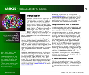
ARTICLE -IntroductionBy Raluca Mihaela Andrei,Mike Panand Monica ZoppèRaluca Mihaela Andrei1,2, MikePan1,* and Monica Zoppè1§1 Scientific Visualization Unit, Institute of Clinical Physiology, CNR ofItaly, Area della Ricerca, Pisa, Italy2 Scuola Normale Superiore, Pisa,Italy* Present address: University of British Columbia, Vancouver, Canada§ Corresponding authorwww.blenderart.org27BioBlender: Blender for BiologistsBiologists know that, if the information oflife is stored and transmitted through nucleic acids (DNA and RNA), the processesthat do the actual work are most of thetimes proteins. These are active in all aspects of life, and in the latest years we arestarting to get a glimpse of how theywork. Proteins are machines composed ofamino acids, which are in turn smallgroups of atoms arranged in specificways[1]. Scientists are obtaining more andmore information on the 3D arrangement of suchatoms, and are starting to understand their activitythrough motion.BioBlender for Windows is available fromwww.bioblender.net (on Linux machines it can beused with Wine). Because of its specialized nature,it requires the installation of PyMOL[3.4] , Python2.6 [5] and NumPy[6] , which are all provided in Installer folder from the downloaded package.Using BioBlender to build an animationTo start BioBlender, simply go to the Bin folder andlaunch blender.exe, then open the template.blendscene (stored in BioBlender folder).Notice that the template file not only has an optimized user-interface layout for biologists, but thetemplate scene also contains lights, camera andworld settings that are ideal for visualizing molecules. This setup ensures that researchers who areOn the basis of information obtained by experinot familiar with the 3D software can still effecments of nuclear magnetic resonance (NMR), 3Dtively use BioBlender. Each interface elementvisualization tools provided by BioBlender allow bi(buttons, sliders, toggles) has help text associatedologists to build a reasonable sequence of movewith it. By placing the mouse over them a pop-upment for proteins. It also includes a dedicated visual text describes the function. Errors and progressescode to represent important features of their surare displayed in the console. Critical errors will apface (Electric and lipophilic potential) on the protein pear in the main BioBlender as a pop-up under theitself, using photo realistic rendering and specialmouse. The atoms size is of order of Ångström (Å),effects.therefore the scale used is 1 Blender Unit 1 Å.BioBlender is a software extension of Blender 2.5[2],an interface for biological visualization that allowsthe user to import and interactively view and manipulate proteins. It was developed and is maintained by the Scientific Visualization Unit of theCNR of Italy in Pisa, with the help and contributionof several members of the Blender community. Material, scenes, publications and other relevant information can be found at www.BioBlender.net and/orwww.scivis.ifc.cnr.it.This tutorial assumes that you already have BioBlender downloaded on your computer, with therequired programs installed.1. Select and import a .pdb filePDB files contain a description of one or multipleconformations (positions) of a single molecule. Different conformations of the same protein are listedin one NMR file and are called MODEL 1, MODEL 2etc.Issue 31 Dec 2010 - "Under the Microscope"

ARTICLE -28BioBlender: Blender for BiologistsA list of options are available to be considered before importing the protein inthe Blender scene (5 in figure):Verbose: enable to display in the console extra information for debugging;SpaceFill: enable or disable to displaythe atoms with Van der Waals or covalent radii in the 3D scene, respectively;In the BioBlender Select PDB File panel: Select the .pdb file by browsing from your data (1in figure). The file included in sampleData foldercontains the 25 models of Calmodulin [7]. Alternatively, simply type the 4-letter code for the .pdb fileto be fetched from www.pdb.org [8] (make sure topick an NMR file);Raluca Mihaela Andrei1,2,Mike Pan1,* and MonicaZoppè1§1 Scientific Visualization Unit,Institute of Clinical Physiology,CNR of Italy, Area della Ricerca, Pisa, Italy2 Scuola Normale Superiore,Pisa, Italy* Present address: Universityof British Columbia, Vancouver, Canada§ Corresponding authorwww.blenderart.org Change the name of the protein (by default it isnamed “protein0”) in the field on the right (2 infigure). Naming the proteins is just a good habitthat will help keeping the scene organized. Once afile is selected, the number of models and thechains are detected and shown in the BioBlenderImport field (3 in figure); Choose 2 models to import in the scene (by defaultall models are listed) typing their number separated by comma; In the Keyframe Interval slider (4 in figure) set thenumber of frames between the protein conformations (Min 1, Max 200).Hydrogen: enable to import Hydrogensif they are present in the .pdb file. Thisoption makes importing much slowerand it is important only for visualization. If the .pdb file does not contain Hydrogens (or ifyou chose not to import them), they will be added during the Electrostatic Potential calculation using external software;Make Bonds: enable it to have atoms connected bychemical bonds. Despite being time consuming thisoperation is very important in motion calculation;High quality: displays high-quality atom and surfacegeometries; slow when enabled;Single User: enable to use shared mesh for atoms inGame Engine; slow when enabled;Upload Errors: enable to send us automatically andanonymously an email with the errors you generate.This makes us aware of the problems that arise andhelp us fix them.Finally, press Import PDB button to import the proteinto the 3D scene of Blender. Blender displays the proteinin motion (by linear interpolation between atoms inthe conformations; Esc to stop the animation).Issue 31 Dec 2010 - "Under the Microscope"

ARTICLE -2. Visualization in the 3D viewport3. Protein motion using the physic engineOnce imported, the protein is displayed with all atoms,Hydrogens included (if the Hydrogens check-box wasenabled). The first 4 buttons in the BioBlender Viewenable different views: only alpha Carbons, main chain(N, CA, C), main chain and side chains (no H), or allatoms.To calculate the transition of the protein between the 2conformations the Blender Physics Engine is used. PressRun in Game Engine button to see the transition. PressEsc to leave GE and then 0 on Numerical Board to seefrom the camera point of view.If the Surface display mode is selected, BioBlender willcompute the surface of the protein by invoking PyMOLsoftware, an external application. It uses the SolventRadius set by the user and returns the Connolly mesh[9], displayed on the BioBlender 3D view. The defaultradius (1.4 Å) is the standard probe sphere, equivalentto water molecules.Raluca Mihaela Andrei1,2,Mike Pan1,* and MonicaZoppè1§1 Scientific Visualization Unit,Institute of Clinical Physiology,CNR of Italy, Area della Ricerca, Pisa, Italy2 Scuola Normale Superiore,Pisa, Italy* Present address: Universityof British Columbia, Vancouver, Canada§ Corresponding authorwww.blenderart.org29BioBlender: Blender for BiologistsTo check the appearance of surface calculated with different solvent radii, change the solvent radius valueand press refresh button. The current surface is deletedand a new one is created.When atoms are displayed, by selecting one atom inthe 3D display, the protein information of the selectedatom is printed in the area outlined below; in the 3Dview the selection will extend to the other atoms of hecorresponding aminoacid.Hit Run in Game Engine button again for an interactively view. When inside the Game Engine, the mousecontrols the rotation of the protein, allowing to inspectthe protein from all angles. The also applies an ambient occlusion filter to the scene, giving the viewer amuch better sense of depth.Set the Collision mode to one of the following states: 0,1 or 2. When set to 0 the transition between the conformations is done using linear interpolation; the atomswill simply move from one position to the other. Whenset to 1 the collisions between atoms are considered,resulting in a more physico-chemical accuratesimulation[10].When set to 2, the newly evaluated movement will berecord to F-Curves. Go to the Timeline panel on Blenderand see that the new conformations are recorded atdifferent time (200 frames away from the last modelimported) as shown in the figure below; in this wayboth sets of transitions are available for comparison.These conformations can be exported as described laterin section 6.Issue 31 Dec 2010 - "Under the Microscope"

ARTICLE -30BioBlender: Blender for Biologistsprocess is alsotime consumingThis visualization method is a novel way to see the MLP and it always refers to lastvalues of a protein onto the surface. Normally this is achanges in therelatively time consuming and tedious process involvMLP grey-levelsing running different programs from the commandvisualization.line, but BioBlender simplifies the entire process by alWhen the calculalowing the user to do everything under one unified intion is done (theterface.button is reIn BioBlender MLP Visualization section:leased) press F12on your keyboard. Choose a Formula (1 in figure; Testa formula [11] isNote:This is the MLPset by default);4. Molecular Lipophilic Potential Visualization Set the Grid Spacing (2 in figure; expressed in Å,lower is more accurate but slower) for MLP calculation;Raluca Mihaela Andrei1,2,Mike Pan1,* and MonicaZoppè1§1 Scientific Visualization Unit,Institute of Clinical Physiology,CNR of Italy, Area della Ricerca, Pisa, Italy2 Scuola Normale Superiore,Pisa, Italy* Present address: Universityof British Columbia, Vancouver, Canada§ Corresponding authorwww.blenderart.org Press Show MLP on Surface. It may take some timeas the MLP is calculated in every point of the grid inthe protein space, then mapped on the surface ofthe protein and finally visualized as levels of grey(light areas for hydrophobic and dark areas for hydrophilic [12]).A typical protein has varying degrees of lipophilicitydistributed on its surface, as shown here for CaM.Use Contrast and Brightness sliders to enhance theMLP representation of your protein. Once you are satisfied with thegrey-levelsvisualizationhit RenderMLP to Surface buttonfor the photorealisticrender. Thisrepresentation usingour novel code: arange of visual features that goes fromshiny-smooth surfaces for hydrophobicareas to dull-roughsurfaces for hydrophilic ones. Thelevels of grey arebaked as image texture that is mapped on specular of the material.A second image is created by adding noise to the first one and mapit on bump. The light areas become shiny and smooth while thedark ones dull and rough as shown in the figure.Press Esc to go back to the Blender scene.5. Electrostatic Potential VisualizationEP is represented as a series of particles flowing alongfield lines calculated according to the potential fielddue to the charges on the protein surface. For this reason, it is necessary to perform a series of steps (as described in [12]), and to decide the physical parametersto be used in the calculation (2 in the figure).Issue 31 Dec 2010 - "Under the Microscope"