Transcription
GPGPU Benchmark Suites:How Well Do They Sample the Performance Spectrum?Jee Ho Ryoo, Saddam J. Quirem, Michael LeBeane, Reena Panda, Shuang Song and Lizy K. JohnThe University of Texas at Austin{jr45842, saddam.quirem, mlebeane, reena.panda, songshuang1990}@utexas.edu, ljohn@ece.utexas.eduAbstractmicroarchitectures, covering a large amount of variance in theperformance spectrum [15, 16, 32]. However, many benchmarks may exhibit similar behaviors from performance perspectives [8]. In CPU benchmarking such as SPEC CPU2006,each time a new suite is released, a committee ensures thatbenchmarks show distinct behaviors and that the suite hasa large coverage in performance spectrum [35]. However,GPGPU benchmarks have not been gone through such a rigorous process prior to release. Thus, they are prone to beingduplicates of existing benchmarks in some other suites or verysimilar to each other. In this situation, some methodologicalguidance can be beneficial to indicate which benchmarks areredundant and which ones form a unique group of workloadsto evaluate GPGPUs.Recently, GPGPUs have positioned themselves in the mainstream processor arena with their potential to perform a massive number of jobs in parallel. At the same time, manyGPGPU benchmark suites have been proposed to evaluate theperformance of GPGPUs. Both academia and industry havebeen introducing new sets of benchmarks each year while somealready published benchmarks have been updated periodically.However, some benchmark suites contain benchmarks that areduplicates of each other or use the same underlying algorithm.This results in an excess of workloads in the same performancespectrum.In this paper, we provide a methodology to obtain a setof new GPGPU benchmarks that are located in the unexplored region of the performance spectrum. Our proposal usesstatistical methods to understand the performance spectrumcoverage and uniqueness of existing benchmark suites. Laterwe show techniques to identify areas that are not exploredby existing benchmarks by visually showing the performancespectrum coverage. Finding unique key metrics for futurebenchmarks to broaden its performance spectrum coverageis also explored using hierarchical clustering and ranking byHotelling’s T2 method. Finally, key metrics are categorizedinto GPGPU performance related components to show howfuture benchmarks can stress each of the categorized metricsto distinguish themselves in the performance spectrum. Ourmethodology can serve as a performance spectrum orientedguidebook for designing future GPGPU benchmarks.This paper uses various statistical methods to evaluateexisting benchmarks in the GPGPU domain. We showthe distribution of existing benchmarks using PrincipalComponent Analysis to locate them in the performancespectrum and suggest where future benchmarks can explore.In order to achieve this, we present methods to identify uniquebenchmarks and their key metrics that exercise extreme endsof the spectrum. Then, we categorize these metrics intodifferent GPGPU performance related components as this willillustrate how a new benchmark with metrics in one isolatedGPGPU component can be used to stress an unexploredperformance spectrum region. Using data collected from realhardware, we investigate which direction new benchmarksshould stress. This paper makes the following contributions:1. Introduction1. We provide a methodology for future GPGPU benchmarksto increase the performance spectrum coverage.2. We perform various statistical analyses to show the suitewise coverage on the performance spectrum and identifykey performance coverage areas that are not explored byexisting suites.3. We use hierarchical clustering and ranking to identifyunique benchmarks that are located at extremes of theperformance spectrum. These benchmarks contain manydistinctive features that can guide the future benchmarksuites to be unique.4. We analyze a very large set of benchmarks (88 benchmarksfrom 5 different benchmark suites) that are widely usedin the GPGPU performance evaluation domain. To ourGPU architects and designers need diverse GPGPU benchmarks in order to guide their designs. As of today, thereare more than 100 GPGPU benchmarks from different suitesavailable on the web for the public. The number of benchmarks in each suite vary from a few to more than fifty. Somesuites are geared toward testing one domain of applicationswhile others attempt to address a large range of applications [13, 30, 31, 37, 38]. The number of GPGPU benchmarks have been rising at a fast pace as newer GPGPUbenchmarks are released every year at various researchvenues [3, 6, 9, 13, 36].On one hand, this large number of benchmarks can helpresearchers stress various components of their proposed future1
SMSMSMSMGPCGPCSHARED MEMORY/L1 CACHETEXTEXTEXTEXTEXTURE CACHEPC14SMPC13SMPC1SMPC12INTERCONNECT ORE/ALUPIPELINECORE/ALUPIPELINEL2 CACHEPC10DISPATCHREGISTER FILEPC9WARP C4MCVariance CoverageWARP TION CACHEPC2DRAMFigure 2: Variance Coverage of PCsFigure 1: GPU Architecture Overviewber of warps in each CTA. The order in which the CTAsexecute is non-deterministic [18]. Besides the fact that theyare able to share the memory, threads within a CTA are ableto synchronize with other threads in the CTA using a barrierinstruction. The GPU will attempt to schedule as many warpsas possible in the same SM. The ratio between number ofwarps executing on an SM and the maximum number of warpswhich can execute on an SM is known as warp occupancy.Threads within a warp can diverge from each other resulting ininactive SIMD lanes. There exists two types of divergence inGPU SIMD architectures, control-flow divergence and memory divergence [33]. Control-flow divergence is the result ofa thread within a warp taking a different path than the otherthreads in the same warp. Memory divergence is the resultof an uncoalesced memory operation where the memory locations accessed by the threads in a warp are unaligned and/ornot adjacent.knowledge, no prior work has explored such a completebenchmark space due to lengthy simulation time as well asinfrastructure issues.The rest of this paper is organized as follows. Section 2provides the background of GPU microarchitectural and programming model. Section 3 provides the overview of ourexperimental setup and methodology while we evaluate ourresults in Section 4. We perform the component-wise studyin Section 5. Section 6 discusses prior work done in this area,and we provide the concluding remarks in Section 8.2. Background2.1. GPU Architecture and Programming ModelFigure 1 displays an overview of a typical GPU’s microarchitecture [24]. The processing cores of the GPU are organizedin Graphics Processing Clusters (GPCs), each of which contains a set of Streaming Multiprocessors (SMs) [12]. All SMsshare a common L2 cache, which is the Last Level Cache(LLC). The SM contains dual warp-schedulers where a warp,a group of 32 threads, executes in SIMT fashion [24, 25].Warp instructions can be dispatched to the core/ALU pipeline,load/store pipeline, or Special Function Unit (SFU) pipelineas shown in the right side of Figure 1. The memory subsystem has a unique type of memory known as shared memory.The name refers the fact that this memory is shared by allthreads in the same Cooperative Thread Array (CTA). Thesize of the CTA is a programmer configurable parameter. Insome architectures, the programmer has the capability to sacrifice L1 cache capacity in favor of a larger shared memory orvice-versa. Besides the L1 cache, a texture cache is used formemory accesses with high spatial locality while a constantcache is used for memory accesses with high temporal locality.Such an architecture is coupled with heterogeneous languages such as OpenCL and CUDA [1, 25]. The languagecreates an abstraction of hardware structures present in theGPU. The programmer has control over the number of threadsthat are launched for a particular kernel by passing the numberof CTAs, known as thread blocks in CUDA and work-groupsin OpenCL. Then, the runtime hardware determines the num-2.2. Principal Component AnalysisIn this section, we explain the Principal Component Analysis (PCA) technique, which is used throughout the paper toshow the distribution of workloads among different benchmark suites in the performance spectrum [11]. PCA convertsi variables X1 , X2 , ., Xi into j linearly uncorrelated variablesXˆ1 , Xˆ2 , ., X̂ j , called Principal Components (PCs). Each Principal Component is a linear combination of the various variables(characteristics) weighted with a certain coefficient, known asthe loading factor, as shown in Equation 1. It has an interestingproperty that the first PC covers the most variance (informationfrom the original data) while the second PC covers the secondmost variance (PC1 contains the most amount of informationabout the data). In this work, we have a total of 14 PCs withthe individual and the cumulative variance coverage shown inFigure 2.iXˆ1 a1k Xkk 1iXˆ2 a2k Xk···(1)k 13. MethodologyThe applications were selected from a set of suites whichare widely used for GPGPU performance evaluation. In this2
Table 1: GPGPU Workload SourcesWorkload SuiteNVIDIA ial VersionInitial VersionTable 3: Description of MetricsMetric# of Applications39219712REPLAY OVERHEADBRANCH EFFWARP EXEC EFFLOAD STORE INSTTable 2: Experimental Platform SpecificationsName#SMProcessor CoresGraphics Clock (MHz)Processor Clock (MHz)L2 Cache Capacity (KB)DRAM InterfaceDRAM Capacity (GB)DRAM Bandwidth (GB/s)Peak GFLOPsValue73848221645512GDDR51.281281263.4CONTROL INSTFP INSTMISC INSTSHARED LDST INSTDP FLOP PKITEX MPKIDRAM WRPKIsection, we discuss these GPGPU application suites in termsof how the various application metrics are collected, how thebenchmarks are selected, and what program characteristics areselected for workload characterization.L1 MISS RATEL2 L1 MISS RATETEX MISS RATEDescriptionAverage number of replays for each 1K instructions executedRatio of non-divergent branches to totalbranchesRatio of the average active threads per warpto the maximum number of threads per warpsupported on a multiprocessor expressed aspercentage (SIMD efficiency)Compute load/store instructions executedby non-predicated threads per total instructions executedControl-flow instructions executed by nonpredicated threads per total instructions executedFloating point instructions executed per total instructions executedMiscellaneous instructions executed per total instructions executedShared load/store instructions executed pertotal instructions executedDouble-precision floating-point operationsexecuted by non-predicated threads per 1Kinstructions executedTexture cache misses per 1K instructions executedDevice memory write transactions per 1Kinstructions executedMiss rate at L1 cacheMiss rate at L2 cache for all read requestsfrom L1 cacheTexture cache miss ratea logarithmic scale in Figure 3. Our evaluation was done onhardware, so the total number of instructions are significantlyhigher than the prior work done on a simulator [12]. Longerexecution time with more representative input sizes can accurately depict the performance characteristics of these GPGPUapplications.3.1. WorkloadsWe use 5 benchmark suites listed in Table 1. For completeness of the analysis, every application in all suites isincluded in the analysis regardless of whether one suite hasa similar benchmark to another suite. For example, we runtwo versions of the histogram-generating applications fromboth the CUDA SDK and Parboil suite. Our workload suitesinclude the widely used Rodinia benchmark suite, the Parboil benchmark suite, the GPGPU-Sim suite presented atISPASS-2009, the Mars MapReduce framework sample applications, and the sample applications included with theCUDA SDK [3, 6, 7, 13, 22, 36]. The largest number of workloads come from the CUDA SDK sample applications whichcover the graphics (MAND), image-processing (DXTC), financial (BS), and simulation (NBODY) domains. The Rodiniaand Parboil suites aim for diversity in the benchmarks. TheGPGPU-Sim and NVIDIA SDK suites are designed for demonstration purposes, while at the same time, providing diversityin their workloads. The Mars sample applications are verysimilar to each other in terms of their code and algorithmsbecause they all depend on a map reduce framework.A large body of simulation based workload characterizationuses reduced input set sizes or shorter runs due to slower simulation speed. In our work, all workloads are executed untilcompletion with representative input sizes. Figure 3 shows thenumber of warp instructions in all benchmarks that are usedin our study. The number of warp instruction counts rangefrom 36,822 in DWTHAAR to 43 billion in CFD. Due to alarge variance in the number of instructions executed, we use3.2. Experimental SetupThe program metrics listed in Table 3 are collected usingwith NVIDIA’s CUDA (6.0) profiler, known as nvprof, on anNVIDIA GTX 560 Ti GPU [23,26]. Table 2 lists detailed specifications of our underlying hardware platform. The programmetrics are collected from reproducible runs of each application. The profiler is capable of retrieving multiple metrics byreplaying GPU kernels.4. Evaluation4.1. GPGPU Workload CharacteristicsThe complexity and diversity of GPGPU workloads continue to increase as they now are tackling larger problems andexpanding across various fields. In order to analyze performance in such workloads, we perform analysis on a comprehensive set of program characteristics. Table 3 provides a listof the performance metrics used in this paper. The total number of dynamic instructions are used to scale many metricsin order to eliminate effects caused by a different number ofinstructions. For example, the total number of texture cachemisses is divided by 1000 instructions to show the miss rateper kilo-instruction (TEX MPKI).3
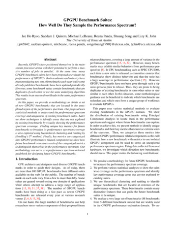
AESB NCILSTEREOSTOSTRMVECADDVIDDECVOLFLTRWCWPNumber of Warp Instructions1.00E 111.00E 101.00E 091.00E 081.00E 071.00E 061.00E 051.00E 041.00E 031.00E 021.00E 011.00E 00Figure 3: Number of Executed Instructions (Logarithmic Scale)PC1PC2PC3with the largest number of benchmarks. Many benchmarkslie on the right side of the scatterplot. The PC1 axis, whereWARP EXEC EFF has the highest weight, controls the horizontal placement, meaning the benchmark suite has manybenchmarks with high SIMD efficiency. Other metrics withhigh PC1 factor loading are BRANCH EFF and FP INST,which are common factors that result in high performance inGPGPUs. This suite is a good representative of GPGPU applications with optimized control flow patterns as they reduceinefficiencies caused by not fully utilizing the available SIMDlanes. Also, a high number of floating point operations usuallyindicate a compute intensive workload, and GPGPUs processthese operations very efficiently. At the same time, this meansthat the suite is missing a set of workloads that are memoryintensive as well as highly control divergent. Figure 5b showsthat this suite is distributed in a narrow region on the PC3 axis,which is dominated by DP FLOP PKI and DRAM WRPKI.The suite does not have a set of benchmarks that extensivelyexercise the DRAM. Figure 5d shows the coverage map ofeach suite. It is noticeable that the width of the CUDA SDKsuite is rather narrow.TEX MISS RATEL2 L1 MISS RATEL1 MISS RATEDRAM WRPKITEX MPKIDP FLOP PKISHARED LDST INSTFP INSTMISC INSTCONTROL INSTLOAD STORE INSTWARP EXEC EFFBRANCH EFFREPLAY OVERHEAD10.80.60.40.20-0.2-0.4-0.6-0.8-1PC4Figure 4: Factor LoadingThe PCA algorithm projects each data point onto the newaxis, the PC. This is done by multiplying each metric by anappropriately weight, called factor loading. The weightedmetrics are then summed to compute each PC. The weightscan show which metrics have significance in each PC. Figure 4shows the weight of each metric on first four PCs. For example,WARP EXEC EFF, BRANCH EFF and FP INST are themetrics that affect PC1. Those metrics with the high PC1factor loading are key metrics that distinguish benchmarksamong each other since PC1 covers the most variance. Insubsequent sections, we will use this background knowledgeto explain various results in detail.Rodinia, on the other hand, covers the left half of PC1 inFigure 5a, which almost complements the missing area ofthe CUDA SDK. This is a good example of how two different suites can yield different results when both suites do nothave a large coverage. For example, if a future architecturewith mores registers were proposed to improves the warp occupancy, CUDA SDK would not see much benefit as mostbenchmarks already have high warp occupancy. Yet, the Rodinia will see significant benefits as the suite is composedof many benchmarks with low warp occupancy. In this case,depending on which suite is used, the outcome can be drastically different and the decision for future architectures maychange. Rodinia covers a wide spectrum in Figure 5d withmany benchmarks being located at different extreme pointsof the coverage envelop. These PC axis show the memoryintensiveness such as cache misses and DRAM accesses, illustrating that this suite has a variety mix of benchmarks thatstress the memory subsystem in different ways.4.2. Performance Spectrum CoverageWe evaluate with the PC scatterplot where each benchmarkis located in the two-dimensional performance spectrum. Figure 5 visually shows the position of each benchmark and thesuite-wise coverage map in the performance spectrum. We donot label each data point to avoid cluttering the plot. However,we will explicitly mention the name of some interesting benchmarks in subsequent sections. Figure 5a shows the scatterplotfor PC1 and PC2. These two PCs cover approximately 35%of the variance as previously shown in Figure 2.The CUDA SDK suite has the most number of data pointsGPGPU-Sim only has 12 benchmarks in the suite, yet thePC1 and PC2 coverage in Figure 5c is rather large. Those4
432211PC4PC234CUDA SDKRodiniaParboilMarsGPGPU Sim00 1 1 2 2 3 3 4 5 4 3 2 1PC10123 4 4CUDA SDKRodiniaParboilMarsGPGPU Sim 202PC34(a) PC1 and PC2(b) PC3 and PC4(c) PC1 and PC2 Coverage Area(d) PC3 and PC4 Coverage Area68Figure 5: Scatterplot Showing 4 PCsbenchmarks are well spread out in the control flow spectrumsince one benchmark has high SIMD efficiency while another shows low SIMD efficiency. This suite not only coversa large spectrum in the control flow space, but also in thememory space as in Figure 5d. L2 L1 MISS RATE andL1 MISS RATE have high weights in the PC4 factor loading,representing memory intensive workloads. This suite stretchesvertically with a good mix of workloads that show both highand low cache misses.Parboil has a small number of benchmarks, yet their performance spectrum lies completely inside the CUDA SDK’sspectrum as seen in Figure 5c and Figure 5d. The suite triesto cover a large area as the coverage spectrum is not narrowin one particular axis direction. This attempt is shown in Figure 5a and Figure 5b as all data points are not clustered in oneregion, but rather, set apart out from each other. Yet, it doesnot exercise any component to the extreme, so the area thatthis suite covers in the spectrum is relatively small. With future processors that improve such bottlenecks as cache misses,it is possible that the spectrum coverage will shrink furthersince metrics such as L1 MISS RATE will decrease. However, it is possible that the existing benchmarks can increasethe coverage area with some improvements. For instance, themetrics that affect Figure 5a are efficiency metrics such as theSIMD efficiency. The lack of hardware resources within theSM usually affects these metrics, so if the program uses moreregisters per thread or has more divergent branches, this willdrag a few of the Parboil benchmarks to the lower end of thespectrum in PC1. Similarly, the input size of the applicationcan be made larger so that it can generate more memory related events such as cache misses. This will eventually leadsome benchmarks to extreme points in Figure 5d.The Mars benchmark suite is designed to use the same mapreduce framework, so their coverage is expected to be smallas shown in Figure 5. This suite is enclosed completely bythe Rodinia suite. If this suite can cover an area that is notcovered by any other suites, then it can stand out as a veryunique benchmark suite. This suite lies near the border of theRodinia coverage envelop, so if it can be stretched little farthertowards one extreme, it can cover its own unique space. In the5
case of Figure 5c, this will be towards the negative end of thePC1 axis. This means that if one of the benchmarks containsslightly lower SIMD efficiency, it can be located outside theRodinia envelop.In Figure 5, many areas are still left to be explored. Especially, the area with positive PC3 and negative PC4 is oneexample. This area corresponds to high floating point instructions, high DRAM read accesses, and high texture cachemisses. A new benchmark to explore this area can be proposedwith a high number of floating point instructions. The textureand L2 misses can be increased by increasing the texture cacheworking set size. Therefore, if a new benchmark is writtenwith these in mind, it can have a large number of read accessesto the texture cache with a large footprint, which eventuallyreaches the DRAM. In addition, the lower PC1 and high PC2area is another unexplored area, which corresponds to lowSIMD efficiency, high load/store instructions and shared load/store instructions. For this area, the future benchmark can bewritten with low SIMD efficiency. Yet, the warp instructionmix in this benchmark can be mainly composed of memoryinstructions. Then, it can eventually fill the missing space inthe performance spectrum.Rodinia-JPEGCUDA SDK-SMOKECUDA SDK-HSOPTParboil-STENCILCUDA SDK-FWTCUDA SDK-SQRNGCUDA SDK-SCANCUDA SDK-VECADDGPGPU-Sim-LPSCUDA SDK-MSORTRodinia-PATHCUDA SDK-BOXFLTRRodinia-HSORTCUDA SDK-MARCUBESCUDA AUSSRodinia-HSPOTRodinia-SRADParboil-SADRodinia-B TREEParboil-SPMVCUDA SDK-PARTCUDA SDK-VIDDECCUDA SDK-CONVFFTCUDA SDK-FLUIDSCUDA im-CUTCP2CUDA SDK-EIGENCUDA SDK-BICUFLTCUDA SDK-CONVTEXCUDA SDK-DENOISECUDA SDK-BILATFLCUDA SDK-VOLFLTRCUDA SDK-BSCUDA SDK-RECGAUSSCUDA SDK-PROCGLGPGPU-Sim-LIBParboil-MRIQCUDA SDK-QRNGMars-MMUL2Rodinia-SCCUDA SDK-REDCUDA SDK-SPCUDA SDK-DCT8X8Parboil-SGEMMGPGPU-Sim-DGParboil-LBMCUDA SDK-MANDCUDA SDK-DXTCCUDA SDK-OCEANRodinia-LEUKOGPGPU-Sim-RAYCUDA SDK-NBODYGPGPU-Sim-AESCUDA SDK-STEREOCUDA SDK-BINOPTCUDA SDK-CONVSEPCUDA SDK-MMULCUDA SDK-FDTD3DRodinia-LUDCUDA HIST2Parboil-MRIGCUDA MUM2Rodinia-MYORodinia-LAVAMD4.3. Similarity/Dissimilarity of BenchmarksWith many data points in the multidimensional PC scatterplot, it is difficult to see similarity between benchmarks.More importantly, if many existing benchmarks are similarto each other, then future benchmarks should be designed tobe dissimilar to those ones in order to place themselves inunexplored areas. The dendrogram can help this process byshowing how similar/dissimilar each benchmark is among 88benchmarks used in this study. A dendrogram is a graphicalrepresentation of the hierarchical clustering method to represent the similarity among benchmarks. First, all metrics inTable 3 are drawn in the multidimensional space. Then, thepairwise distance of all benchmarks is computed and a treeis constructed based on the distance of each pair as shownin Figure 6. If a pair of two benchmarks is very similar, itwill have a short distance, and thus, will be linked at the leafsof the tree (left side of the figure). At the end, a group ofmost dissimilar benchmarks are linked at the root of the tree.Subsetting a large number of benchmarks can easily be donewith the dendrogram. If one wants to determine a subset of2 benchmarks, then draw a vertical line which has two intersections [21]. In our figure, a dotted line drawn at the linkagedistance value of 12 corresponds to this point. One intersection corresponds to the Rodinia-LAVAMD benchmark, and theother intersection corresponds to 87 other benchmarks [27].This means the Rodinia-LAVAMD is the most unique program,and the program at the center of the other subset with the 87programs will be used to represent that subset.In Figure 6, we see that all of the Mars benchmarks arefound to be similar, suggesting that a single map-reduce application is sufficient when used in benchmarking. A similar2468Linkage DistanceFigure 6: Dendrogram61012
NEURALLAVAMDTable 4: Uniqueness Rank of -AESGPGPU-Sim-STOCUDA SDK-MANDParboil-LBMRank910111213141516MYO(a) Rodinia-LAVAMD(b) GPGPU-Sim-NEURALLOAD STORE INSTCONTROL INST LOAD STORE INSTBIT CONV INSTCONTROL INSTresult is shown with the image processing benchmarksBIT CONV INSTofthe CUDA SDK suite, specifically BICUFLT, BILATFL, FP32 INSTDEFP64 INSTINTEGER INST FP64 INSTFP32 INSTINTEGER INSTBIT CONV INSTLOAD STORE INSTCONTROL INSTFP32 INSTNOISE, and CONVTEX. Besides those benchmarks foundinINTER THREAD INSTINTER THREAD INSTMISC INSTFP64 INSTMISC INST INTEGER INSTINTER THREAD INSTMISC INSTthe same domain, some were found to be similar due to theusage of a common algorithm, namely scalar-produce(SP) andFigure 7: Instruction Mix of 2 Most Dissimilar Programsreduction(RED). Parallel reduction is a major phase of scalarproduct calculation.The results indicate that future benchwith the prior finding since the 5 Rodinia benchmarks mademarks need to have workloads that are distinct from imageit in the top 8 list. Although the ranking itself does not showprocessing or map-reduce to be unique in the performancewhich end of the extremes the benchmark exists, the methodspectrum. Also, future benchmarks should avoid using existology we have developed throughout the paper, including theing benchmarks’ algorithms to eliminate redundancy.PC scatterplot, can clearly show where high ranking benchA general goal in benchmarking is to increase the performarks exist in the scatterplot. The top 5 Rodinia benchmarksmance spectrum coverage. A good benchmark suite will haveare located at the edges of the coverage envelop in Figure 5c.a large number of benchmarks that are connected at the rootIn addition, the GPGPU-Sim suite also has 7 benchmarks inof the tree. The dendrogram in Figure 6 can indicate thatthe top 16 list. Although the Parboil and Mars suite have amore types of benchmarks such as Rodinia-LAVAMD andrelatively small number of benchmarks, a few benchmarksGPGPUSim-MUM2 are needed. Not surprisingly, those aresuch as Parboil-LBM and Mars-STRM are included in the topbenchmarks that are located in their unique spaces in the PC16 list as they are located near the edge of the envelop.scatterplot presented in Section 4.2. Therefore, an effectiveUnique benchmarks can help future benchmark designersvisual representation of the dendrogram can drive where newwithimportant architectural components. They can offer inbenchmark efforts should go in the performance spectrum.sights into the source of underlying features that make themunique. Here, we will dive into the three most unique bench4.4. Ranking Benchmarksmarks, LAVAMD, MYO, and NEURAL. LAVAMD is uniqueA new benchmark should target a unique space in the peramong the Rodinia suite as it is the only benchmark repreformance spectrum in order not to overlap with existing benchsenting the N-Body dwarf [2, 27]. This benchmark features amarks or suites. The dendrogram can be effective in showinghigh branch and warp execution efficiency as well as efficienta few unique benchmarks, but with such a large number ofshared memory access patterns. Figure 7a explains anotherbenchmarks, it is hard to illustrate how unique one benchmarkunusual characteristic of Rodinia-LAVAMD as it has a highis relative to another. Especially in our study with 88 benchnumber of miscellaneous instructions, which include barriermarks, choosing unique benchmarks just by looking at theinstructions. Also, the problem size is partitioned to fit indendrogram can be difficult. Hotelling’s T2 method [17] canconstant memory, so the computation is done only within eachhelp identifying unique programs. It is a statistical methodthread block, achieving high SIMD efficiency. However, evento find the most extreme data point in multivariate distributhough MYO is a floating-point benchmark just like LAVAMD,tion. The benchmark that is farthest away from the centerit features very low memory efficiency. Each instance of thisof the distribution is marked as the most unique benchmarkworkload is assigned to a thread, so this workload does notin this study. Ranking benchmarks based on Hotelling’s T2orchestrate memory accesses to take advantage of caches suchhelps us select unique benchmarks when the subsetting theas constant memory. Therefore, this benchmark incurs signifidendrogram results in that one subset contains too many benchcantly more cache misses than others. NEURAL operates onmarks. Table 4 lists the top 16 unique benchmarks
GPGPU-Sim Initial Version 12 Table 2: Experimental Platform Specifications Name Value #SM 7 Processor Cores 384 Graphics Clock (MHz) 822 Processor Clock (MHz) 1645 L2 Cache Capacity (KB) 512 DRAM Interface GDDR5 DRAM Capacity (GB) 1.28 DRAM Bandwidth (GB/s) 128 Peak GFLOPs 1263.4 section, we discuss these GPGPU application suites in terms