WIXLIB

5426423520617814912091321048121620242832(a) A compute-bound 28765421048121632(b) A bandwidth-bound kernel.264235206178149120913202428(c) A balanced kernel.Normalized Performance643.5Normalized Performance7Normalized PerformanceNormalized 2832(d) An irregular kernel.Fig. 1: Four different GPGPU performance scaling surfaces. Frequency is held at 1 GHz while CUs and bandwidth are varied.Advanced reconfiguration systems try to predict the effectof their changes on the total performance of the system. Forinstance, boosting a CPU’s frequency may prevent a nearbyGPU from reaching its optimal operating point, requiring online thermal models to maximize chip-wide performance [42].Similarly, using power and performance estimates to proactively choose the best voltage and frequency state (rather thanreacting only to the results of previous decisions) can enablepower capping solutions, optimize energy usage, and yieldhigher performance in “dark silicon” situations [46], [49].Estimating how applications scale across hardware configurations is a crucial aspect of these systems. These estimatesmust be made rapidly, precluding low-level simulators, andmust react to dynamic program changes, which limits the useof analytic models based on static analyses. We therefore studymodels that quickly estimate power and performance usingeasy-to-obtain dynamic hardware event counters.D. High-Level GPGPU ModelThe recurring theme in these examples is a desire for afast, relatively accurate estimation of performance and powerat different hardware configurations. Previous studies havedescribed high-level models that can predict performance atdifferent frequencies, which can be used for online optimizations [24], [39], [45]. Unfortunately, these systems are limitedby their models designed after abstractions of real hardware.Fig. 1 shows the performance of four OpenCLTM kernels ona real GPU. The performance (Y-axis) changes as the numberof active CUs (X-axis) and the available memory bandwidth(Z-axis) are varied. Frequency is fixed at 1 GHz.Existing models that compare compute and memory workcan easily predict the applications shown in Fig. 1(a) and 1(b)because they are compute and bandwidth-bound, respectively.Fig. 1(c) is more complex; its limiting factor depends on ratioof CUs to bandwidth. This requires a model that handleshardware component interactions [23], [54].Fig. 1(d) shows a performance effect that can be difficultto predict with simple models. Adding more CUs helps performance until a point, whereupon performance drops as moreare added. This is difficult to model using linear regression orsimple compute-versus-bandwidth formulae.As more CUs are added, more pressure is put on the sharedL2 cache. Eventually, the threads’ working sets overflow theL2 cache, degrading performance. This effect has been shownin simulation, but simple analytic models do not take it intoaccount [29], [34]. Numerous other non-obvious scaling resultsexist, but we do not detail them due to space constraints.Suffice to say, simple models have difficulty with kernels thatare constrained by complex microarchitectural limitations.Nevertheless, our goal is to create a high-level modelthat we can use to estimate performance and power acrossa wide range of hardware configurations. As such, we buildan ML model that can perform these predictions quickly andaccurately.We begin by training on a large number of OpenCL kernels.We run each kernel at numerous hardware configurations whilemonitoring power, performance, and hardware performancecounters. This allows us to collect data such as that shownin Fig. 1. We find that the performance and power of manyGPU kernels scale similarly. We therefore cluster similarkernels together and use the performance counter informationto fingerprint that scaling surface.To make predictions for new kernels, we measure theperformance counters obtained from running that kernel at onehardware configuration. We then use them to predict whichscaling surface best describes this kernel. With this, we canquickly estimate the performance or power of a kernel at manyconfigurations. The following section details this process.III.M ETHODOLOGYWe describe our modeling methodology in two passes.First, Section III-A describes the methodology at a high level,providing a conceptual view of how each part fits together.Then Section III-B, Section III-C, and Section III-D go intothe implementation details of the different parts of the model.For simplicity, these sections describe a performance model,but this approach can be applied to generate power models aswell.A. OverviewWhile our methodology is amenable to modeling anyparameter that can be varied, for the purposes of this study, wedefine a GPU’s hardware configuration as its number of CUs,engine frequency, and memory frequency. We take as an inputto our predictor measurements gathered on one specific GPUhardware configuration called the base hardware configuration. Once a kernel has been executed on the base hardwareconfiguration, the model can be used to predict the kernel’sperformance on a range of target hardware configurations.

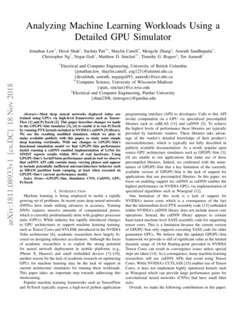
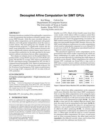
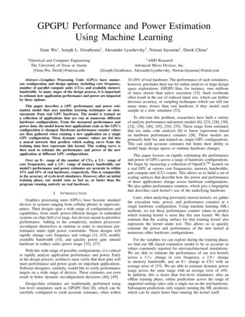
ormanceCountersKernel 3Kernel 4Kernel 5Kernel 6TargetHardwareConfigurationModelTarget ExecutionTime/PowerCluster 1Fig. 2: The model construction and usage flow. Trainingis done on many configurations, while predictions requiremeasurements from only one.CU count,Engine freq., Mem. freq,4,300,375Kernel 2GPU HardwareTraining SetKernel nameKernel 1 32,1000,1375Perf. Count 1.Perf. Count. 2 Cluster 3Cluster 2Fig. 4: Forming clusters of kernel scaling behaviors. Kernelsthat scale in similar ways are clustered together.PerformanceCounter Values(from baseconfiguration)Kernel 1Classifier? .Cluster 1Kernel NExecution Times/PowerCluster 2Cluster 3Performance Counter Values gatheredon base hardware configurationFig. 3: The model’s training set, which contains the performance or power of each training kernel for a range of hardwareconfigurations.The model construction and usage flow are depicted inFig. 2. The construction algorithm uses a training data setcontaining execution times and performance counter valuescollected from executing training kernels on real hardware. Thevalues in the training set are shown in Fig. 3. For each trainingkernel, execution times and performance counter values acrossa range of hardware configurations are stored in the trainingset. The performance counter values collected while executingeach training kernel on the base hardware configuration arealso stored.Once the model is constructed, it can be used to predictthe performance of new kernels, from outside the training set,at any target hardware configuration within the range of thetraining data. To make a prediction, the kernel’s performancecounter values and base execution time must first be gatheredby executing it on the base hardware configuration. These arethen passed to the model, along with the desired target hardware configuration, which will output a predicted executiontime at that target configuration. The model is constructed onceoffline but used many times. It is not necessary to gather atraining set or rebuild the model for every prediction.Model construction consists of two major phases. In thefirst phase, the training kernels are clustered to form groupsof kernels with similar performance scaling behaviors acrosshardware configurations. Each resulting cluster represents onescaling behavior found in the training set.In the simple example shown in Fig. 4, there are six trainingkernels being mapped to three clusters. Training kernels 1and 5 are both bandwidth bound and are therefore mappedFig. 5: Building a classifier to map from performance countervalues to clusters.to the same cluster. Kernel 3 is the only one of the six thatis purely compute bound, and it is mapped to its own cluster.The remaining kernels scale with both compute and memorybandwidth, and they are all mapped to the remaining cluster.While this simple example demonstrates the general approach,the actual model identifies larger numbers of clusters withmore complex scaling behaviors in a 4D space.In the second phase, a classifier is constructed to predictwhich cluster’s scaling behavior best describes a new kernelbased on its performance counter values. The classifier, shownFig. 5, would be used to select between the clusters inFig. 4. The classifier and clusters together allow the modelto predict the scaling behavior of a new kernel across a widerange of hardware configurations using information taken fromexecuting it on the base hardware configuration. When themodel is asked to predict the performance of a new kernel ata target hardware configuration, the classifier is accessed first.The classifier chooses one cluster, and that cluster’s scalingbehavior is used to scale the baseline execution time to thetarget configuration in order to make the desired prediction.Fig. 6 gives a detailed view of the model architecture.Notice that the model contains multiple sets of clusters andclassifiers. Each cluster set and classifier pair is responsiblefor providing scaling behaviors for a subset of the CU,engine frequency, and memory frequency parameter space. Forexample, the top cluster set in Fig. 6 provides informationabout the scaling behavior when CU count is 8. This set provides performance scaling behavior when engine and memoryfrequencies are varied and CU count is fixed at 8. The exact

VariableCU luster2 ClusterN2Target Config.Exec. Time137519258009006007000400ClusterN3500 MemoryFrequency4300Cluster2Normalized PerformanceCluster1 Engine Frequency475MemoryFrequency24281000 ClusterN ClassifierCUs 32set ClassifierCluster23Engine Frequency Performance CounterValues(from assifierCUs 8setNormalized PerformanceBase Config. Exec.Time & Target Config.65432104812162032CU countFig. 6: Detailed architecture of our performance and power predictor. Performance counters from one execution of the applicationare used to find which cluster best represents how this kernel will scale as the hardware configuration is changed. Each clustercontains a scaling surface that describes how this kernel will scale when some hardware parameters are varied.number of sets and classifier pairs in a model depends on thehardware configurations that appear in the training set.The scaling information from these cluster sets allows scaling from the base to any other target configuration. By dividingthe parameter space into multiple regions and clustering thekernels once for each region, the model is given additionalflexibility. Two kernels may have similar scaling behaviors inone region of the hardware configuration space, but differentscaling in another region. For example, two kernels may scaleidentically with respect to engine frequency, but one may notscale at all with CU count while the other scales linearly.For cases like this, the kernels may be clustered together inone cluster set but not necessarily in others. Breaking theparameter space into multiple regions and clustering eachregion independently allows kernels to be grouped into clusterswithout requiring that they scale similarly across the entireparameter space. In addition, by building a classifier for eachregion of the hardware configuration space, each classifier onlyneeds to learn performance counter trends relevant to its region,which reduces their complexity.The remainder of this section provides descriptions ofthe steps required to construct this model. The calculationof scaling values, which are used to describe a kernel’sscaling behavior, is described in Section III-B. Section III-Cdescribes how these are used to form sets of clusters. Finally,Section III-D describes the construction of the neural networkclassifiers.B. Scaling SurfacesOur first step is to convert the training kernel executiontimes into performance scaling values, which capture howthe kernels’ performance changes as the number of CUs,engine frequency, and memory frequency are varied. Scalingvalues are calculated for each training kernel and then putinto the clustering algorithm. Because we want to form groupsof kernels with similar scaling behaviors, even if they havevastly different execution times, the kernels are clustered usingscaling values rather than raw execution times.To calculate scaling values, the training set executiontimes are grouped by kernel. Then, for each training kernel,a 3D matrix of execution times is formed. Each dimensioncorresponds to one of the hardware configuration parameters.In other words, the position of each execution time in thematrix is defined by the number of CUs, engine frequency,and memory frequency combination it corresponds to.The matrix is then split into sub-matrices, each of whichrepresents one region of the parameter space. Splitting thematrix in this way will form the multiple cluster sets seenin Fig. 6. An execution time sub-matrix is formed for eachpossible CU count found in the training data. For example, iftraining set data have been gathered for CU counts of 8, 16,24, and 32, four sub-matrices will be formed per kernel.The process to convert an execution time sub-matrix intoperformance scaling values is illustrated using the example inFig. 7. An execution time sub-matrix with a fixed CU countis shown in Fig. 7(a). Because the specific CU count does notchange any of the calculations, it has not been specified. Inthis example, it is assumed that the training set engine andmemory frequency both range from 400 MHz to 1000 MHzwith a step size of 200 MHz. However, the equations givenapply to any range of frequency values, and the reshaping ofthe example matrices to match the new range of frequencyvalues is straightforward.Two types of scaling values are calculated from the execution times shown in Fig. 7. Memory frequency scalingvalues, shown in Fig. 7(b), capture how execution timeschange as memory frequency increases and engine frequencyremains the same. Engine frequency scaling values, shownin Fig. 7(c), capture how execution times change as enginefrequency increases and memory frequency remains the same.In the memory scaling matrix, each entry’s column positioncorresponds to a change in memory frequency and its rowposition corresponds to a fixed engine frequency. In the enginescaling matrix, each entry’s column position corresponds to achange in engine frequency and its row position correspondsto a fixed memory frequency.

t2,0 t2,1 t2,2 t2,3600t1,0 t1,1 t1,2 t1,3400t0,0 t0,1 t0,2 t0,3𝑚𝑖,𝑗 Mem. Freq. (MHz)(a) Execution times𝑡𝑖,𝑗 1𝑡𝑖,𝑗m3,0 m3,1 m3,2800m2,0 m2,1 m2,2600m1,0 m1,1 m1,2400m0,0 m0,1 m0,2𝑒𝑖,𝑗𝑡𝑖 1,𝑗 𝑡𝑖,𝑗Engine Freq. (MHz)800t3,0 t3,1 t3,2 t3,3Engine Freq. (MHz)Engine Freq. (MHz)10001000Mem. Freq. (MHz)800 to 1000e2,0 e2,1 e2,2 e2,3600 to 800e1,0 e1,1 e1,2 e1,3400 to 600e0,0 e0,1 e0,2 e0,3Mem. Freq. (MHz)(b) Memory frequency scaling values.(c) Engine frequency scaling values.Fig. 7: Calculation of frequency scaling values.As long as the CU counts of the base and target configurations remain the same, one or more of the shown scaling valuescan be multiplied with a base configuration execution time topredict a target configuration execution time. We will showhow to calculate the scaling factors to account for variableCU counts shortly. The example in Equation 1 shows howthese scaling values are applied. The base configuration hasa 400 MHz engine clock and a 400 MHz memory clock.The base execution time is t0,0 . We can predict the targetexecution time, t3,3 , of a target configuration with a 1000MHz engine clock and a 1000 MHz memory clock usingEquation 1. Scaling values can also be used to scale fromhigher frequencies to lower frequencies by multiplying thebase execution time with the reciprocals of the scaling values.For example, because m0,0 can be used to scale from a 400MHz to 600 MHz memory frequency, m10,0 can be used toscale from a 600 MHz to 400 MHz memory frequency. Scalingexecution times in this way may not seem useful when onlytraining data is considered, as the entire execution time matrixis known. However, after the model has been constructed, thesame approach can be used to predict execution times fornew kernels at configurations that have not been run on realhardware.22YYt3,3 t0,0e0,jmi,2(1)j 0i 0In addition to the engine and memory frequency scalingvalues, a set of scaling values is calculated to account forvarying CU count. A sub-matrix, from which CU scalingvalues can be extracted, is constructed. All entries of thisnew sub-matrix correspond to the base configuration engineand memory frequency. However, each entry corresponds toone of the CU counts found in the training data. An exampleexecution time sub-matrix with variable CU count is shown inFig. 8(a). A set of CU scaling behavior values are calculatedusing the template shown in Fig. 8(b).To predict a target configuration execution time, the CUscaling values are always applied before applying any engineor memory frequency scaling values. The difference betweenthe base and target configuration CU counts determines which,if any, CU scaling values are multiplied with the base executiontime. After applying CU scaling values to the base executiontime, the resulting scaled value is further scaled using theCompute UnitsCompute Units8t0162432t1t2t3(a) Execution times.𝑐𝑖 𝑡𝑖 1𝑡𝑖c0c1c2(b) Compute unit scaling values.Fig. 8: Calculation of CU scaling values.memory and engine frequency sets corresponding to the targetCU count. This yields a target execution time that correspondsto the CU count, engine frequency, and memory frequency ofthe target configuration.C. ClusteringK-means clustering is used to create sets of scaling behaviors representative of the training kernels. The training kernelsare clustered multiple times to form multiple sets of clusters.Each time, the kernels are clustered based on a different setof the scaling values discussed in Section III-B. Each set ofclusters is representative of the scaling behavior of one regionof the hardware configuration parameter space. The trainingkernels are clustered once for each CU count available inthe training set hardware configurations and once based ontheir scaling behavior as CU count is varied. For example, i

GPGPU-Sim, for instance, runs millions of times slower than native execution [35]. Such overheads often result in the use of reduced input sets, which can further decrease accuracy, or sampling techniques which can still run many times slower than real hardware if they model each