Transcription
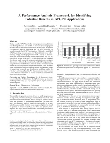
A Performance Analysis Framework for IdentifyingPotential Benefits in GPGPU ApplicationsJaewoong SimAniruddha Dasgupta† Hyesoon KimRichard VuducAbstractTuning code for GPGPU and other emerging many-core platformsis a challenge because few models or tools can precisely pinpointthe root cause of performance bottlenecks. In this paper, we presenta performance analysis framework that can help shed light onsuch bottlenecks for GPGPU applications. Although a handful ofGPGPU profiling tools exist, most of the traditional tools, unfortunately, simply provide programmers with a variety of measurements and metrics obtained by running applications, and it is often difficult to map these metrics to understand the root causes ofslowdowns, much less decide what next optimization step to take toalleviate the bottleneck. In our approach, we first develop an analytical performance model that can precisely predict performance andaims to provide programmer-interpretable metrics. Then, we applystatic and dynamic profiling to instantiate our performance modelfor a particular input code and show how the model can predict thepotential performance benefits. We demonstrate our framework ona suite of micro-benchmarks as well as a variety of computationsextracted from real codes.Categories and Subject Descriptors C.1.4 [Processor Architectures]: Parallel Architectures; C.4 [Performance of Systems]:Modeling techniques; C.5.3 [Computer System Implementation]:MicrocomputersGeneral TermsMeasurement, PerformanceKeywords CUDA, GPGPU architecture, Analytical model, Performance benefit prediction, Performance prediction1. IntroductionWe consider the general problem of how to guide programmersor high-level performance analysis and transformation tools withperformance information that is precise enough to identify, understand, and ultimately fix performance bottlenecks. This paper proposes a performance analysis framework that consists of an analytical model, suitable for intra-node analysis of platforms basedon graphics co-processors (GPUs), and static and dynamic profiling tools. We argue that our framework is suitable for performance The work was done while the author was at Georgia Institute of Technology.Permission to make digital or hard copies of all or part of this work for personal orclassroom use is granted without fee provided that copies are not made or distributedfor profit or commercial advantage and that copies bear this notice and the full citationon the first page. To copy otherwise, to republish, to post on servers or to redistributeto lists, requires prior specific permission and/or a fee.PPoPP’12, February 25–29, 2012, New Orleans, Louisiana, USA.c 2012 ACM 978-1-4503-1160-1/12/02. . . 10.00Copyright Normalized PerformanceGeorgia Institute of TechnologyPower and Performance Optimization Labs, AMD†{jaewoong.sim, hyesoon.kim, .41.210.80.60.40.20Baseline SharedMemorySFUTightOne OptimizationUJAMShared Shared SharedMemory Memory Memory SFU Tight UJAMShared Memory AnotherFigure 1. Performance speedup when some combinations of fourindependent optimization techniques are applied to a baseline kernel.diagnostics through examples and case studies on real codes andsystems.Consider an experiment in which we have a computational kernel implemented on a GPU and a set of n independent candidateoptimizations that we can apply. Figure 1 shows the normalizedperformance when some combinations of four independent optimization techniques are applied to such a kernel, as detailed in Section 6.2.1. The leftmost bar is the parallelized baseline. The nextfour bars show the performance of the kernel with exactly one offour optimizations applied. The remaining bars show the speedupwhen one more optimization is applied on top of Shared M emory ,one of the optimizations.The figure shows that each of four optimizations improves performance over the baseline, thereby making them worth applying to the baseline kernel. However, most of programmers cannot estimate the degree of benefit of each optimization. Thus, aprogrammer is generally left to use intuition and heuristics. Here,Shared M emory optimization is a reasonable heuristic startingpoint, as it addresses the memory hierarchy.Now imagine a programmer who, having applied SharedM emory , wants to try one more optimization. If each optimizationis designed to address a particular bottleneck or resource constraint,then the key to selecting the next optimization is to understand towhat extent each bottleneck or resource constraint affects the current code. In our view, few, if any, current metrics and tools forGPUs provide this kind of guidance. For instance, the widely usedoccupancy metric on GPUs indicates only the degree of threadlevel parallelism (TLP), but not the degree of memory-level orinstruction-level parallelism (MLP or ILP).In our example, the kernel would not be improved muchif the programmer tries the occupancy-enhancing T ight sinceShared M emory has already removed the same bottleneck that
T ight would have. On the other hand, if the programmer decides toapply SF U , which makes use of special function units (SFUs)in the GPU, the kernel would be significantly improved sinceShared Memory cannot obtain the benefit that can be achievedby SF U .Our proposed framework, GPUPerf, tries to provide such understanding. GPUPerf quantitatively estimates potential performancebenefits along four dimensions: inter-thread instruction-level parallelism (Bitilp ), memory-level parallelism (Bmemlp ), computing efficiency (Bfp ), and serialization effects (Bserial ). These four metricssuggest what types of optimizations programmers (or even compilers) should try first.GPUPerf has three components: a frontend data collector, ananalytical model, and a performance advisor. Figure 2 summarizes the framework. GPUPerf takes a CUDA kernel as an input and passes the input to the frontend data collector. The frontend data collector performs static and dynamic profiling to obtain a variety of information that is fed into our GPGPU analyticalmodel. The analytical model greatly extends an existing model, theMWP-CWP model [9], with support for a new GPGPU architecture(“Fermi”) and addresses other limitations. The performance advisor digests the model information and provides interpretable metrics to understand potential performance bottlenecks. That is, byinspecting particular terms or factors in the model, a programmeror an automated tool could, at least in principle, use the informationdirectly to diagnose a bottleneck and perhaps prescribe a tor#instsILP, enefit metricsFigure 2. An overview of GPUPerf.For clarity, this paper presents the framework in a “reverse order.” It first describes the key potential benefit metrics output bythe performance advisor to motivate the model, then explains theGPGPU analytical model, and lastly explains the detailed mechanisms of the frontend data collector. After that, to evaluate theframework, we apply it to six different computational kernels and44 different optimizations for a particular computation. Furthermore, we carry out these evaluations on actual GPGPU hardware,based on the newest NVIDIA C2050 (“Fermi”) system. The resultsshow that our framework successfully differentiates the effects ofvarious optimizations while providing interpretable metrics for potential bottlenecks.In summary, our key contributions are as follows:1. We present a comprehensive performance analysis framework,GPUPerf, that can be used to predict performance and understand bottlenecks for GPGPU applications.2. We propose a simple yet powerful analytical model that is anenhanced version of the MWP-CWP model [9]. Specifically,we focus on improving the differentiability across distinct optimization techniques. In addition, by following the work-depthgraph formalism, our model provides a way to interpret modelcomponents and relates them directly to performance bottlenecks.3. We propose several new metrics to predict potential performance benefits.2. MWP-CWP ModelThe analytical model developed for GPUPerf is based on the onethat uses MWP and CWP [9]. We refer to this model as the MWPCWP model in this paper. The MWP-CWP model takes the following inputs: the number of instructions, the number of memoryrequests, and memory access patterns, along with GPGPU architecture parameters such as DRAM latency and bandwidth. The total execution time for a given kernel is predicted based on the inputs. Although the model predicts execution cost fairly well, theunderstanding of performance bottlenecks from the model is not sostraightforward. This is one of the major motivations of GPUPerf.2.1 Background on the MWP-CWP ModelFigure 3 shows the MWP-CWP model. The detailed descriptionsof the model can be found in [9]. Here, we breifly describe thekey concepts of the model. The equations of MWP and CWPcalculations are also presented in Appendix A.1113252476181MWP 82233434MWP 25456CWP 5OneMemoryWaitingPeriod5676778One ComputationPeriodComputation Period8CWP 58Memory PeriodFigure 3. MWP-CWP model. (left: MWP CWP, right: MWP CWP)Memory Warp Parallelism (MWP): MWP represents themaximum number of warps2 per streaming multiprocessor (SM) 3that can access the memory simultaneously. MWP is an indicatorof memory-level parallelism that can be exploited but augmentedto reflect GPGPU SIMD execution characteristics. MWP is a function of the memory bandwidth, certain parameters of memory operations such as latency, and the number of active warps in anSM. Roughly, the cost of memory operations is modeled to be thenumber of memory requests over MWP. Hence, modeling MWPcorrectly is very critical.Computation Warp Parallelism (CWP): CWP represents thenumber of warps that can finish their one computation period during one memory waiting period plus one. For example, in Figure 3,CWP is 5 in both cases. One computation period is simply theaverage computation cycles per one memory instruction. CWP ismainly used to classify three cases, which are explained below.Three Cases: The key component of the MWP-CWP modelis identifying how much (and/or which) cost can be hidden bymulti-threading in GPGPUs. Depending on the relationship between MWP and CWP, the MWP-CWP model classifies the threecases described below.1. MWP CWP: The cost of computation is hidden by memoryoperations, as shown in the left figure. The total execution costis determined by memory operations.2. MWP CWP: The cost of memory operations is hidden bycomputation, as shown in the right figure. The total executioncost is the sum of computation cost and one memory period.3. Not enough warps: Due to the lack of parallelism, both computation and memory operation costs are only partially hidden.2.2 Improvements over the MWP-CWP ModelAlthough the baseline model provides good prediction results formost GPGPU applications, some limitations make the model oblivious to certain optimization techniques. For instance, it assumes1 MWP and CWP calculations are updated for the analytical model inGPUPerf.2 Warp, a group of 32 threads, is a unit of execution in a GPGPU.3 SM and core are used interchangeably in this paper.
3. Performance AdvisorThe goal of the performance advisor is to convey performance bottleneck information and estimate the potential gains from reducingor eliminating these bottlenecks. It does so through four potentialbenefit metrics, whose impact can be visualized using a chart asillustrated by Figure 4. The x-axis shows the cost of memory operations and the y-axis shows the cost of computation. An application code is a point on this chart (here, point A). The sum of thex-axis and y-axis values is the execution cost, but because computation and memory costs can be overlapped, the final execution costof Texec (e.g., wallclock time) is a different point, A’, shifted relative to A. The shift amount is denoted as Toverlap . A diagonal linethrough y x divides the chart into compute bound and memorybound zones, indicating whether an application is limited by computation or memory operations, respectively. From point A’, thebenefit chart shows how each of the four different potential benefitmetrics moves the application execution time in this space.A given algorithm may be further characterized by two additional values. The first is the ideal computation cost, which is generally the minimum time to execute all of the essential computational work (e.g., floating point operations), denoted Tfp in Figure 4. The second is the minimum time to move all data from theDRAM to the cores, denoted by Tmem min . When memory requestsare prefetched or all memory service is hidden by other computation, we might hope to hide or perhaps eliminate all of the memory operation costs. Ideally, an algorithm designer or programmercould provide estimates or bounds on Tfp and Tmem min . However,4 PTX is an intermediate representation used before register allocation andinstruction scheduling.Compute Bound ZoneA’BmemlpTcompToverlapABserialComputation Costthat a memory instruction is always followed by consecutive dependent instructions; hence, MLP is always one. Also, it ideallyassumes that there is enough instruction-level parallelism. Thus, itis difficult to predict the effect of prefetching or other optimizationsthat increase instruction/memory-level parallelism.Cache Effect: Recent GPGPU architectures such as NVIDIA’sFermi GPGPUs have a hardware-managed cache memory hierarchy. Since the baseline model does not model cache effects, thetotal memory cycles are determined by multiplying memory requests and the average global memory latency. We simply modelthe cache effect by calculating average memory access latency(AMAT); the total memory cycles are calculated by multiplyingmemory requests and AMAT.SFU Instruction: In GPGPUs, expensive math operations suchas transcendentals and square roots can be handled with dedicatedexecution units called special function units (SFUs). Since theexecution of SFU instructions can be overlapped with other floatingpoint (FP) instructions, with a good ratio between SFU and FPinstructions, the cost of SFU instructions can almost be hidden.Otherwise, SFU contention can hurt performance. We model thesecharacteristics of special function units.Parallelism: The baseline model assumes that ILP and TLP areenough to hide instruction latency, thereby using the peak instruction throughput when calculating computation cycles. However,when ILP and TLP are not high enough to hide the pipeline latency,the effective instruction throughput is less than the peak value. Inaddition, we incorporate the MLP effect into the new model. MLPcan reduce total memory cycles.Binary-level Analysis: The MWP-CWP model only uses information at the PTX level.4 Since there are code optimization phasesafter the PTX code generation, using only the PTX-level information prevents precise modeling. We develop static analysis tools toextract the binary-level information and also utilize hardware performance counters to address this issue.BitilpBfpMemory Bound ZoneTfpTmem minTmem’TmemMemory CostPotential ImprovementFigure 4. Potential performance benefits, illustrated.when the information is not available, we could try to estimate Tfpfrom, say, the number of executed FP instructions in the kernel.5Suppose that we have a kernel, at point A’, having differentkinds of inefficiencies. Our computed benefit factors aim to quantify the degree of improvement possible through the elimination ofthese inefficiencies. We use four potential benefit metrics, summarized as follows. Bitilp indicates the potential benefit by increasing inter-threadinstruction-level parallelism. Bmemlp indicates the potential benefit by increasing memory-level parallelism. Bfp represents the potential benefit when we ideally removethe cost of inefficient computation. Unlike other benefits, wecannot achieve the 100% of Bfp because a kernel must havesome operations such as data movements. Bserial shows the amount of savings when we get rid of theoverhead due to serialization effects such as synchronizationand resource contention.Bitilp , Bfp , and Bserial are related to the computation cost, whileBmemlp is associated with the memory cost. These metrics aresummarized in Table 1.NameTexecTcompTmemToverlap TmemTfpTmem minBserialBitilpBmemlpBfpDescriptionFinal predicted execution timeComputation costMemory costOverlapped cost due to multi-threadingTmem ToverlapIdeal TcompIdeal TmemBenefits of removing serialization effectsBenefits of increasing inter-thread ILPBenefits of increasing MLPBenefits of improving computing efficiencyUnitcostcostcostcostcostideal costideal costbenefitbenefitbenefitbenefitTable 1. Summary of performance guidance metrics.5 In our evaluation we also use the number of FP operations to calculate T .fp
4. GPGPU Analytical ModelIn this section we present an analytical model to generate theperformance metrics described in Section 3. The input parametersto the analytical model are summarized in Table 2.4.1 Performance PredictionFirst, we define Texec as the overall execution time, which is afunction of Tcomp , Tmem , and Toverlap , as shown in Equation (1).Texec Tcomp Tmem Toverlap(1)As illustrated in Figure 4, the execution time is calculated byadding computation and memory costs while subtracting the overlapped cost due to the multi-threading feature in GPGPUs. Each ofthe three inputs of Equation (1) is described in the following.Synchronization Overhead, Osync : When there is a synchronization point, the instructions after the synchronization point cannot be executed until all the threads reach the point. If all threadsare making the same progress, there would be little overhead forthe waiting time. Unfortunately, each thread (warp) makes its ownprogress based on the availability of source operands; a range ofprogress exists and sometimes it could be wide. The causes ofthis range are mainly different DRAM access latencies (delayingin queues, DRAM row buffer hit/miss etc.) and control-flow divergences. As a result, when a high number of memory instructionsand synchronization instructions exist, the overhead increases asshown in Equations (7) and (8):4.1.1 Calculating the Computation Cost, TcompOsync Fsync Tcomp is the amount of time to execute compute instructions (ex-cluding memory operation waiting time, but including the costof executing memory instructions) and is evaluated using Equations (2) through (10).We consider the computation cost as two components, a parallelizable base execution time plus overhead costs due to serialization effects:Tcomp Wparallel Wserial .(2) Base OverheadThe base time, Wparallel , accounts for the number of operations anddegree of parallelism, and is computed from basic instruction andhardware values as shown in Equation (3):Wparallel #insts #total warps avg inst lat .#active SMs ITILP(3)ITILPITILPmax min (ILP N, ITILPmax )(4) avg inst lat,warp size/SIMD width(5)where N is the number of active warps on one SM, and SIMD widthand warp size represent the number of vector units and the number of threads per warp, respectively. On the Fermi architecture,SIMD width warp size 32. ITILP cannot be greater thanITILPmax , which is the ITILP required to fully hide pipeline latency.We model serialization overheads, Wserial from Equation (2), asWserial Osync OSFU OCFdiv Obank ,(6)where each of the four terms represents a source of overhead—synchronization, SFU resource contention, control-flow divergence, and shared memory bank conflicts. We describe each overhead below.(7)(8)Mem. ratiowhere Γ is a machine-dependent parameter. We chose 64 for themodeled architecture based on microarchitecture simulations.SFU Resource Contention Overhead, OSFU : This cost ismainly caused by the characteristics of special function units(SFUs) and is computed using Equations (9) and (10) below. Asdescribed in Section 2.2, the visible execution cost of SFU instructions depends on the ratio of SFU instructions to others andthe number of execution units for each instruction type. In Equation (9), the visibility is modeled by FSFU , which is in [0, 1]. A valueof FSFU 0 means none of the SFU execution costs is added to thetotal execution time. This occurs when the SFU instruction ratio isless than the ratio of special function to SIMD units as shown inEquation (10).Total instructions per SM Effective throughputThe first factor in Equation (3) is the total number of instructionsthat an SM executes, and the second factor indicates the effectiveinstruction throughput. Regarding the latter, the average instructionlatency, avg inst lat, can be approximated by the latency of FP operations in GPGPUs. When necessary, it can also be precisely calculated by taking into account the instruction mix and the latencyof individual instructions on the underlying hardware. The value,ITILP, models the possibility of inter-thread instruction-level parallelism in GPGPUs. In particular, instructions may issue from multiple warps on a GPGPU; thus, we consider global ILP (i.e., ILPamong warps) rather than warp-local ILP (i.e., ILP of one warp).That is, ITILP represents how much ILP is available among all executing to hide the pipeline latency.ITILP can be obtained as follows:#sync insts #total warps Fsync#active SMs#mem instsΓ avg DRAM lat , #insts OSFU #SFU insts #total warpswarp size FSFU#active SMsSFU width SFU throughputFSFU min max #SFU insts #insts (9) SFU width,0 ,1 . SIMD width SFU inst. ratio SFU exec. unit ratio(10)Control-Flow Divergence and Bank Conflict Overheads,OCFdiv and Obank : The overhead of control-flow divergence (OCFdiv )is the cost of executing additional instructions due, for instance, todivergent branches [9]. This cost is modeled by counting all theinstructions in both paths. The cost of bank conflicts (Obank ) canbe calculated by measuring the number of shared memory bankconflicts. Both OCFdiv and Obank can be measured using hardwarecounters. However, for control-flow divergence, we use our instruction analyzer (Section 5.2), which provides more detailed statistics.4.1.2 Calculating the Memory Access Cost, TmemTmem represents the amount of time spent on memory requests andtransfers. This cost is a function of the number of memory requests,memory latency per each request, and the degree of memory-levelparallelism. We model Tmem using Equation (11),Tmem #mem insts #total warps AMAT,#active SMs ITMLP Effective memory requests per SM(11)
where AMAT models the average memory access time, accountingfor cache effects. We compute AMAT using Equations (12) and (13): AMATavg DRAM lat avg DRAM lat miss ratio hit lat (12)DRAM lat (avg trans warp 1) Δ.(13)Model Parameter#insts#mem insts#sync insts#SFU insts#FP insts#total warps#active SMsNavg DRAM lat represents the average DRAM access latency andis a function of the baseline DRAM access latency, DRAM lat,and transaction departure delay, Δ. In GPGPUs, memory requestscan split into multiple transactions. In our model, avg trans warprepresents the average number of transactions per memory requestin a warp. Note that it is possible to expand Equation (12) formultiple levels of cache, which we omit for brevity.We model the degree of memory-level parallelism through anotion of inter-thread MLP, denoted ITMLP, which we define as thenumber of memory requests per SM that is concurrently serviced.Similar to ITILP, memory requests from different warps can beoverlapped. Since MLP is an indicator of intra-warp memory-levelparallelism, we need to consider the overlap factor of multiplewarps. ITMLP can be calculated using Equations (14) and (15).ITMLP min MLP MWPcp , MWPpeak bwMWPcp min (max (1, CWP 1) , MWP) AMATavg trans warpavg inst latmiss ratiosize of dataILPMLPMWP (Per SM)CWP (Per SM)MWPpeak bw (Per SM)warp sizeΓΔDRAM latFP lathit latSIMD widthSFU width(14)Table 2. Summary of input parameters used in equations.memory performance (time). Alternatively, an algorithm developermight provide these estimates.#FP insts #total warps FP latTfp #active SMs ITILP(18)size of data avg DRAM latTmem min (19)MWPpeak bwThen, the benefit metrics are obtained using Equations (20)-(23),where ITILPmax is defined in Equation (5):4.1.3 Calculating the Overlapped Cost, ToverlapToverlap represents how much the memory access cost can be hiddenby multi-threading. In the GPGPU execution, when a warp issuesa memory request and waits for the requested data, the executionis switched to another warp. Hence, Tcomp and Tmem can be overlapped to some extent. For instance, if multi-threading hides allmemory access costs, Toverlap will equal Tmem . That is, in this casethe overall execution time, Texec , is solely determined by the computation cost, Tcomp . By contrast, if none of the memory accessescan be hidden in the worst case, then Toverlap is 0.We compute Toverlap using Equations (16) and (17). In theseequations, Foverlap approximates how much Tcomp and Tmem overlap and N represents the number of active warps per SM as in Equation (4). Note that Foverlap varies with both MWP and CWP. WhenCWP is greater than MWP (e.g., an application limited by memoryoperations), then Foverlap becomes 1, which means all of Tcomp canbe overlapped with Tmem . On the other hand, when MWP is greaterthan CWP (e.g., an application limited by computation), only partof computation costs can be overlapped. Foverlap min(Tcomp Foverlap , Tmem ) N ζ1 (CWP MWP), ζ N0 (CWP MWP)SourceSec. 5.1Sec. 5.1Sec. 5.2Sec. 5.2Sec. 5.2Sec. 5.1Sec. 5.1Sec. 5.1Sec. 5.1Sec. 5.2Sec. 5.2Sec. 5.1source codeSec. 5.3Sec. 5.3Appx.AAppx.AAppx.A3264Table 3Table 3Table 3Table 3Table 3Table 3(15)In Equation (14), MWPcp represents the number of warps whosememory requests are overlapped during one computation period.As described in Section 2.1, MWP represents the maximum number of warps that can simultaneously access memory. However, depending on CWP, the number of warps that can concurrently issuememory requests is limited.MWPpeak bw represents the number of memory warps per SMunder peak memory bandwidth. Since the value is equivalent to themaximum number of memory requests attainable per SM, ITMLPcannot be greater than MWPpeak bw .ToverlapDefinition# of total insts. per warp (excluding SFU insts.)# of memory insts. per warp# of synchronization insts. per warp# of SFU insts. per warp# of floating point insts. per warpTotal number warps in a kernel# of active SMs# of concurrently running warps on one SMAverage memory access latencyAverage memory transactions per memory requestAverage instruction latencyCache miss ratioThe size of input dataInst.-level parallelism in one warpMemory-level parallelism in one warpMax #warps that can concurrently access memory# of warps executed during one mem. period plus oneMWP under peak memory BW# of threads per warpMachine parameter for sync costTransaction departure delayBaseline DRAM access latencyFP instruction latencyCache hit latency# of scalar processors (SPs) per SM# of special function units (SFUs) per SM(16)(17)4.2 Potential Benefit PredictionAs discussed in Section 3, the potential benefit metrics indicateperformance improvements when it is possible to eliminate thedelta between the ideal performance and the current performance.Equations (18) and (19) are used to estimate the ideal compute and5.Bitilp Bserial Bfp #insts #total warps avg inst lat#active SMs ITILPmax(20)Wserial(21)Tcomp Tfp Bitilp Bserial(22)Bmemlp (23)Wparallel max Tmem Tmem min , 0 .Frontend Data CollectorAs described in Section 4, the GPGPU analytical model requires avariety of information on the actual binary execution. In our framework, the frontend data collector does the best in accurately obtaining various types of information that instantiates the analyticalmodel. For this purpose, the frontend data collector uses three different tools/ways to extract the information: compute visual profiler, instruction analyzer (IA), and static analysis tools, as shownin Figure 5.CUDA ExecutableComputeVisual Profiler#insts,occupancy, .Ocelot ExecutableInstructionAnalyzer (IA)#SFU insts, .CUDA Binary(CUBIN)Static AnalysisToolsILP, MLP, .To AnalyticalModelFigure 5. Frontend data collector.
5.1 Compute Visual ProfilerWe use Compute Visual Profiler [14] to access GPU hardware performance counters. It provides accurate architecture-related information: occupancy, total number of global load/store requests, thenumber of registers used in a thread, the number of DRAM reads/writes and cache hits/misses.5.2 Instruction AnalyzerAlthough the hardware performance counters provide accurate runtime information, we still cannot obtain some crucial information.For example, instruction category information, which is essentialfor considering the effects of synchronization and the overhead ofSFU utilization, is not available.Our instruction analyzer module is based on Ocelot [6], a dynamic compilation framework that emulates PTX execution. Theinstruction analyzer collects instruction mixture (SFU, Sync, andFP instructions) and loop information such as loop trip counts. Theloop information is used to combine static analysis from CUDA binary (CUBIN) files and run-time execution information. Althoughthere is code optimization from PTX to CUBIN, we observe thatmost loop information still remains the same.5.3 Static Analysis ToolsOur static analysis tools work on PTX, CUBIN and the informationfrom IA. The main motivation for using static analysis is to obtainILP and MLP information in binaries rather than in PTX code.Due to instruction scheduling and register allocation, which areperformed during target code generation, the degree of parallelismbetween PTX and CUBIN can be significantly di
Potential Benefits in GPGPU Applications Jaewoong Sim Aniruddha Dasgupta† Hyesoon Kim Richard Vuduc Georgia Institute of Technology Power and Performance Optimization Labs, AMD† {jaewoong.sim, hyesoon.kim, riche}@gatech.edu aniruddha.dasgupta@amd.com Abstract Tuning code for GPGPU and other emerging many-core platforms