WIXLIB

12R. S. SUTTONprediction learning, and we refer to learning methods that take this approachas supervised-learning methods. We argue that such methods are inadequate,and that TD methods are far preferable.2.1 Single-step and multi-step predictionTo clarify this claim, we distinguish two kinds of prediction-learning problems. In single-step prediction problems, all information about the correctnessof each prediction is revealed at once. In multi-step prediction problems, correctness is not revealed until more than one step after the prediction is made,but partial information relevant to its correctness is revealed at each step.For example, the weather prediction problem mentioned above is a multi-stepprediction problem because inconclusive evidence relevant to the correctnessof Monday's prediction becomes available in the form of new observations onTuesday, Wednesday, Thursday and Friday. On the other hand, if each day'sweather were to be predicted on the basis of the previous day's observations that is, on Monday predict Tuesday's weather, on Tuesday predict Wednesday'sweather, etc. - one would have a single-step prediction problem, assuming nofurther observations were made between the time of each day's prediction andits confirmation or refutation on the following day.In this paper, we will be concerned only with multi-step prediction problems.In single-step problems, data naturally comes in observation-outcome pairs;these problems are ideally suited to the pairwise supervised-learning approach.Temporal-difference methods cannot be distinguished from supervised-learningmethods in this case; thus the former improve over conventional methods onlyon multi-step problems. However, we argue that these predominate in realworld applications. For example, predictions about next year's economic performance are not confirmed or disconfirmed all at once, but rather bit by bitas the economic situation is observed through the year. The likely outcomeof elections is updated with each new poll, and the likely outcome of a chessgame is updated with each move. When a baseball batter predicts whether apitch will be a strike, he updates his prediction continuously during the ball'sflight.In fact, many problems that are classically cast as single-step predictionproblems are more naturally viewed as multi-step problems. Perceptual learning problems, such as vision or speech recognition, are classically treated assupervised learning, using a training set of isolated, correctly-classified inputpatterns. When humans hear or see things, on the other hand, they receive astream of input over time and constantly update their hypotheses about whatthey are seeing or hearing. People are faced not with a single-step problem ofunrelated pattern-class pairs, but rather with a series of related patterns, allproviding information about the same classification. To disregard this structure seems improvident.2.2 Computational issuesIn this subsection, we introduce a particular TD procedure by formally relating it to a classical supervised-learning procedure, the Widrow-Hoff rule.

TEMPORAL-DIFFERENCE LEARNING13We show that the two procedures produce exactly the same weight changes,but that the TD procedure can be implemented incrementally and thereforerequires far less computational power. In the following subsection, this TDprocedure will be used also as a conceptual bridge to a larger family of TDprocedures that produce different weight changes than any supervised-learningmethod. First, we detail the representational assumptions that will be usedthroughout the paper.We consider multi-step prediction problems in which experience comes inobservation-outcome sequences of the form x1, x2, x 3 ,., xm, z, where each xtis a vector of observations available at time t in the sequence, and z is theoutcome of the sequence. Many such sequences will normally be experienced.The components of each Xt are assumed to be real-valued measurements orfeatures, and z is assumed to be a real-valued scalar. For each observationoutcome sequence, the learner produces a corresponding sequence of predictions P1 , P2,P3, , Pm, each of which is an estimate of z. In general, each Ptcan be a function of all preceding observation vectors up through time t, but,for simplicity, here we assume that it is a function only of X t . 1 The predictionsare also based on a vector of modifiable parameters or weights, w. Pt's functional dependence on xt and w will sometimes be denoted explicitly by writingit as P(xt,w).All learning procedures will be expressed as rules for updating w. For themoment we assume that w is updated only once for each complete observationoutcome sequence and thus does not change during a sequence. For eachobservation, an.increment to w, denoted Aw t , is determined. After a completesequence has been processed, w is changed by (the sum of) all the sequence'sincrements:Later, we will consider more incremental cases in which w is updated aftereach observation, and also less incremental cases in which it is updated onlyafter accumulating Awt's over a training set consisting of several sequences.The supervised-learning approach treats each sequence of observations andits outcome as a sequence of observation-outcome pairs; that is, as the pairs(x1, z), (x2, z),., (xm, z). The increment due to time t depends on the errorbetween Pt and z, and on how changing w will affect Pt. The prototypicalsupervised-learning update procedure iswhere a is a positive parameter affecting the rate of learning, and the gradient,VwPt, is the vector of partial derivatives of Pt with respect to each componentof w.For example, consider the special case in which Pt is a linear function of xtand w, that is, in which Pt wTxt E i w(i)x t (i), where w(i) and xt(i) are'The other cases can be reduced to this one by reorganizing the observations in such away that each xt includes some or all of the earlier observations. Cases in which predictionsshould depend on t can also be reduced to this one by including t as a component of xt.

R. S. SUTTON14the i'th components of w and Xt, respectively.2 In this case we have VwPt Xt,and (2) reduces to the well known Widrow-Hoff rule (Widrow & Hoff, 1960):This linear learning method is also known as the "delta rule," the ADALINE,and the LMS filter. It is widely used in connectionism, pattern recognition,signal processing, and adaptive control. The basic idea is that the differencez - w T x t represents the scalar error between the prediction, w T x t , and whatit should have been, z. This is multiplied by the observation vector xt todetermine the weight changes because xt indicates how changing each weightwill affect the error. For example, if the error is positive and xt(i) is positive,then Wi(t) will be increased, increasing wTxt and reducing the error. TheWidrow-Hoff rule is simple, effective, and robust. Its theory is also betterdeveloped than that of any other learning method (e.g., see Widrow & Stearns,1985).Another instance of the prototypical supervised-learning procedure is the"generalized delta rule," or backpropagation procedure, of Rumelhart et al.(1985). In this case, Pt is computed by a multi-layer connectionist networkand is a nonlinear function of xt and w. Nevertheless, the update rule usedis still exactly (2), just as in the Widrow-Hoff rule, the only difference beingthat a more complicated process is used to compute the gradient VwPt.In any case, note that all Awt in (2) depend critically on z, and thus cannotbe determined until the end of the sequence when z becomes known. Thus,all observations and predictions made during a sequence must be remembereduntil its end, when all the Aw t 's are computed. In other words, (2) cannot becomputed incrementally.There is, however, a TD procedure that produces exactly the same resultas (2), and yet which can be computed incrementally. The key is to representthe error z — Pt as a sum of changes in predictions, that is, aswhereUsing this, equations (1) and (2) can be combined as2 Tw is the transpose of the column vector w. Unless otherwise noted, all vectors arecolumn vectors.

TEMPORAL-DIFFERENCE LEARNING15In other words, converting back to a rule to be used with (1):Unlike (2), this equation can be computed incrementally, because each Awtdepends only on a pair of successive predictions and on the sum of all pastvalues for VwPt. This saves substantially on memory, because it is no longernecessary to individually remember all past values of VwPt. Equation (3) alsomakes much milder demands on the computational speed of the device thatimplements it; although it requires slightly more arithmetic operations overall(the additional ones are those needed to accumulate E k 1 V w P k ) , they canbe distributed over time more evenly. Whereas (3) computes one incrementto w on each time step, (2) must wait until a sequence is completed and thencompute all of the increments due to that sequence. If M is the maximumpossible length of a sequence, then under many circumstances (3) will requireonly 1/Mth of the memory and speed required by (2).3For reasons that will be made clear shortly, we refer to the procedure givenby (3) as the TD(1) procedure. In addition, we will refer to a procedure aslinear if its predictions Pt are a linear function of the observation vectors xtand the vector of memory parameters w, that is, if Pt wTXt .We have justproven:Theorem 1 On multi-step prediction problems, the linear TD(1) procedureproduces the same per-sequence weight changes as the Widrow-Hoff procedure.Next, we introduce a family of TD procedures that produce weight changesdifferent from those of any supervised-learning procedure.2.3 The TD(A) family of learning proceduresThe hallmark of temporal-difference methods is their sensitivity to changesin successive predictions rather than to overall error between predictions andthe final outcome. In response to an increase (decrease) in prediction from Ptto P t 1 , an increment Awt is determined that increases (decreases) the predictions for some or all of the preceding observation vectors x 1 , . . . , xt. Theprocedure given by (3) is the special case in which all of those predictions arealtered to an equal extent. In this article we also consider a class of TD procedures that make greater alterations to more recent predictions. In particular,we consider an exponential weighting with recency, in which alterations to thepredictions of observation vectors occurring k steps in the past are weightedaccording to Ak for 0 A 1:3Strictly speaking, there are other incremental procedures for implementing the combination of (l) and (2), but only the TD rule (3) is appropriate for updating w on aper-observation basis.

16R. S. SUTTONNote that for A 1 this is equivalent to (3), the TD implementation of the prototypical supervised-learning method. Accordingly, we call this new procedureTD(A) and we will refer to the procedure given by (3) as TD(1).Alterations of past predictions can be weighted in ways other than the exponential form given above, and this may be appropriate for particular applications. However, an important advantage to the exponential form is that itcan be computed incrementally. Given that et is the value of the sum in (4)for t, we can incrementally compute e t 1 , using only current information, asFor A 1, TD(A) produces weight changes different from those made by anysupervised-learning method. The difference is greatest in the case of TD(0)(where A 0), in which the weight increment is determined only by its effecton the prediction associated with the most recent observation:Note that this procedure is formally very similar to the prototypical supervisedlearning procedure (2). The two equations are identical except that the actualoutcome z in (2) is replaced by the next prediction Pt 1 in the equation above.The two methods use the same learning mechanism, but with different errors.Because of these relationships and TD(0)'s overall simplicity, it is an importantfocus here.3. Examples of faster learning with TD methodsIn this section we begin to address the claim that TD methods make moreefficient use of their experience than do supervised-learning methods, that theyconverge more rapidly and make more accurate predictions along the way. TDmethods have this advantage whenever the data sequences have a certain statistical structure that is ubiquitous in prediction problems. This structurenaturally arises whenever the data sequences are generated by a dynamicalsystem, that is, by a system that has a state which evolves and is partially revealed over time. Almost any real system is a dynamical system, including theweather, national economies, and chess games. In this section, we develop twoillustrative examples: a game-playing example to help develop intuitions, anda random-walk example as a simple demonstration with experimental results.3.1 A game-playing exampleIt seems counter-intuitive that TD methods might learn more efficiently thansupervised-learning methods. In learning to predict an outcome, how can one

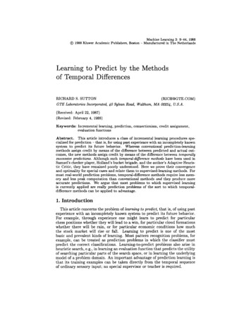
TEMPORAL-DIFFERENCE LEARNING17Figure 1 A game-playing example showing the inefficiency of supervised-learningmethods. Each circle represents a position or class of positions from a twoperson board game. The "bad" position is known from long experience tolead 90% of the time to a loss and only 10% of the time to a win. The firstgame in which the "novel" position occurs evolves as shown by the dashedarrows. What evaluation should the novel position receive as a result ofthis experience? Whereas TD methods correctly conclude that it shouldbe considered another bad state, supervised-learning methods associate itfully with winning, the only outcome that has followed it.do better than by knowing and using the actual outcome as a performancestandard? How can using a biased and potentially inaccurate subsequent prediction possibly be a better use of the experience? The following example ismeant to provide an intuitive understanding of how this is possible.Suppose there is a game position that you have learned is bad for you, thathas resulted most of the time in a loss and only rarely in a win for your side. Forexample, this position might be a backgammon race in which you are behind,or a disadvantageous configuration of cards in blackjack. Figure 1 representsa simple case of such a position as a single "bad" state that has led 90% ofthe time to a loss and only 10% of the tune to a win. Now suppose you playa game that reaches a novel position (one that you have never seen before),that then progresses to reach the bad state, and that finally ends neverthelessin a victory for you. That is, over several moves it follows the path shownby dashed lines in Figure 1. As a result of this experience, your opinion ofthe bad state would presumably improve, but what of the novel state? Whatvalue would you associate with it as a result of this experience?A supervised-learning method would form a pair from the novel state andthe win that followed it, and would conclude that the novel state is likely tolead to a win. A TD method, on the other hand, would form a pair fromthe novel state and the bad state that immediately followed it, and wouldconclude that the novel state is also a bad one, that it is likely to lead to a

18R. S. SUTTONFigure 2. A generator of bounded random walks. This Markov process generated thedata sequences in the example. All walks begin in state D. From statesB, C, D, E, and F, the walk has a 50% chance of moving either to theright or to the left. If either edge state, A or G, is entered, then the walkterminates.loss. Assuming we have properly classified the "bad" state, the TD method'sconclusion is the correct one; the novel state led to a position that you knowusually leads to defeat; what happened after that is irrelevant. Although bothmethods should converge to the same evaluations with infinite experience, theTD method learns a better evaluation from this limited experience.The TD method's prediction would also be better had the game been lostafter reaching the bad state, as is more likely. In this case, a supervisedlearning method would tend to associate the novel position fully with losing,whereas a TD method would tend to associate it with the bad position's 90%chance of losing, again a presumably more accurate assessment. In either case,by adjusting its evaluation of the novel state towards the bad state's evaluation,rather than towards the actual outcome, the TD method makes better use ofthe experience. The bad state's evaluation is a better performance standardbecause it is uncorrupted by random factors that subsequently influence thefinal outcome. It is by eliminating this source of noise that TD methods canoutperform supervised-learning procedures.In this example, we have ignored the possibility that the bad state's previously learned evaluation is in error. Such errors will inevitably exist and willaffect the efficiency of TD methods in ways that cannot easily be evaluatedin an example of this sort. The example does not prove TD methods will bebetter on balance, but it does demonstrate that a subsequent prediction caneasily be a better performance standard than the actual outcome.This game-playing example can also be used to show how TD methods canfail. Suppose the bad state is usually followed by defeats except when it ispreceded by the novel state, in which case it always leads to a victory. Inthis odd case, TD methods could not perform better and might perform worsethan supervised-learning methods. Although there are several techniques foreliminating or minimizing this sort of problem, it remains a greater difficultyfor TD methods than it does for supervised-learning methods. TD methodstry to take advantage of the information provided by the temporal sequenceof states, whereas supervised-learning methods ignore it. It is possible for thisinformation to be misleading, but more often it should be helpful.

TEMPORAL-DIFFERENCE LEARNING19Finally, note that although this example involved learning an evaluationfunction, nothing about it was specific to evaluation functions. The methodscan equally well be used to predict outcomes unrelated to the player's goals,such as the number of pieces left at the end of the game. If TD methods aremore efficient than supervised-learning methods in learning evaluation functions, then they should also be more efficient in general prediction-learningproblems.3.2 A random-walk exampleThe game-play ing example is too complex to analyze in great detail. Previous experiments with TD methods have also used complex domains (e.g.,Samuel, 1959; Sutton, 1984; Barto et al., 1983; Anderson, 1986, 1987). Whichaspects of these domains can be simplified or eliminated, and which aspectsare essential in order for TD methods to be effective? In this paper, we propose that the only required characteristic is that the system predicted be adynamical one, that it have a, state which can be observed evolving over time.If this is true, then TD methods should leam more efficiently than supervisedlearning methods even on very simple prediction problems, and this is what weillustrate in this subsection. Our example is one of the simplest of dynamicalsystems, that which generates bounded random walks.A bounded random walk is a state sequence generated by taking randomsteps to the right or to the left until a boundary is reached. Figure 2 shows asystem that generates such state sequences. Every walk begins in the centerstate D. At each step the walk moves to a neighboring state, either to the rightor to the left with equal probability. If either edge state (A or G) is entered,the walk terminates. A typical walk might be DCDEFG. Suppose we wishto estimate the probabilities of a walk ending in the rightmost state, G, giventhat it is in each of the other states.We applied linear supervised-learning and TD methods to this problem ina straightforward way. A walk's outcome was defined to be z 0 for a walkending on the left at A and z 1 for a walk ending on the right at G.The learning methods estimated the expected value of z; for this choice ofz, its expected value is equal to the probability of a right-side termination.For each nonterminal state i, there was a corresponding observation vectorXi; if the walk was in state i at time t then xt xi. Thus, if the walkDCDEFG occurred, then the learning procedure would be given the sequenceX D , X C , X D , X F ; , X F , 1- The vectors {xi} were the unit basis vectors of length5, that is, four of their compon

the stock market will rise or fall. Learning to predict is one of the most basic and prevalent kinds of learning. Most pattern recognition problems, for . or checker game outcomes. Here we advocate viewing TD methods in a simpler way - as methods for efficiently learning to predict arbitrary events, not just goal-related ones. This simplifica-