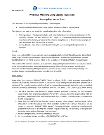
Transcription
Stats 170A: Project in Data SciencePredictive Modeling: RegressionPadhraic SmythDepartment of Computer ScienceBren School of Information and Computer SciencesUniversity of California, Irvine
Reading, Homework, Lectures Reference reading:Chapters 1, 2 and 4 in Geron’s text, Hands-On Machine Learning with ScikitLearn and TensorFlow Homework 6– Will be announced shortly– Will be due by 2pm Wednesday next week (Monday is a holiday) Next Lectures––––Today: prediction with regressionWednesday: prediction with classificationWednesday next week: text analysis and classificationLikely to be 1 more homework (#7) and then project modePadhraic Smyth, UC Irvine: Stats 170AB, Winter 2018: 2
Data Science: from Data to ploratoryData ictiveModelingDataManagementDatabases, Algorithms,Software EngineeringGovernmentScientistsMachine Learning,StatisticsDomain knowledgeBusiness knowledgePadhraic Smyth, UC Irvine: Stats 170AB, Winter 2018: 3
Basic Principles of Predictive ModelingReference reading:Chapters 1, 2 and 4 in Geron’s text, Hands-On Machine Learning withScikit-Learn and TensorFlowPadhraic Smyth, UC Irvine: Stats 170AB, Winter 2018: 4
Predictive Modeling Two basic types of predictive models– Regression: predict a real-valued variable Y given input vector X E.g., predict what a customer will spend with a merchant in the next 12months– Classification: predict a categorical variable Y give input vector X E.g., predict if a credit card transaction is fraudulent or not Both problems can be addressed by statistical or machine learningapproaches Both problems share common mathematical/statistical foundationsPadhraic Smyth, UC Irvine: Stats 170AB, Winter 2018: 5
Learning a Regression 001262126252007197618150011250 000114521981220082000250000Training 8450Data 960060.0014260 84.00Learning algorithm learns a function that takes feature valueson the left to predict the target value on the rightPadhraic Smyth, UC Irvine: Stats 170AB, Winter 2018: 6
Learning a Regression 001262126252007197618150011250 00014260 reaMoSoldYrSoldYearBuiltSalePrice11200 70.0010401040220081965?11924 85.0011822324720062005?Training 8450Data 9600TestData60.00LotFrontageWe can then use the model to make predictionswhen target values are unknownPadhraic Smyth, UC Irvine: Stats 170AB, Winter 2018: 7
Machine Learning NotationFeaturesxinputs to the modelTargetsytarget value we would like to predictPredictions ŷ f(x, w)model’s prediction given inputs x and weights wParameters α or wweights, coefficients specifying the modelErrorerror between target and prediction(e.g., squared error)e( y , ŷ )Padhraic Smyth, UC Irvine: Stats 170AB, Winter 2018: 8
Translating between Statistics and Machine LearningStatisticsMachine LearningParameter estimationLearning algorithmCoefficients, parametersWeightsCovariates, independent variablesInputs, features, attributesDependent variableTargetPadhraic Smyth, UC Irvine: Stats 170AB, Winter 2018: 9
Regression Y is real-valued– E.g., Y can take values y from - to , or y from 0 to , etc Typical applications–––––Predicting how many items of a particular type Amazon will need in 6 monthsPredicting how many times a Facebook user will login in the next monthPredicting how much a house will sell forPredicting the value of Dow Jones Index by end of day tomorrow and so onPadhraic Smyth, UC Irvine: Stats 170AB, Winter 2018: 10
Classification Y is categorical– e.g., Y is binary, takes values y in {0, 1} Many applications––––Predict if an email is spam or not based on its contentPredict what word a person spoke given an audio signalPredict if a moving object in an image is a person or not . Classification is closely related to regression– Similar underlying mathematical principles(sidenote: mathematically, both are trying to predict E[ y x ]– In classification its often very useful to predict p(y 1 x), i.e. a real-valuednumber between 0 and 1 (rather just a hard decision)Padhraic Smyth, UC Irvine: Stats 170AB, Winter 2018: 11
Machine Learning Algorithms: A Component ViewPrediction Model Loss Function Optimization MethodThe functional formof f( x w ), e.g., weightedlinear sum, decision tree, The “algorithm” that finds theparameters w that minimize theerror function, e.g., solving a setof linear equations, gradientdescent, etcHow we measure the quality of themodel’s predictions for specificparameter settings w, e.g., squarederror, absolute error, Padhraic Smyth, UC Irvine: Stats 170AB, Winter 2018: 12
Linear ModelA linear model computes a weighted sum of the inputse.g., in 2 dimensions (2 input features)f(x, w) predicted output w0 w1 x1 w2 x2Why do we need this extra constant weight?More generally, with an arbitrary number of input featuresf(x, w) w0 Σj wj xj w0 wT xPadhraic Smyth, UC Irvine: Stats 170AB, Winter 2018: 13
Optimizing (Minimizing) the Error Function(for squared error and a linear model)E(w ) Σisquared error (ith target, ith prediction) Σi( yi – f (xi ; w) )2 Σi( yi – w0 w1 xi1 w2 xi2 )2How do we minimize this as a function of the weights w?Necessary condition: partial derivative for each weight 0Because this equation is quadratic in the w’s, each partial derivative is linear in wIn the example above, we get 3 simultaneous linear equations (all 0) in 3 unknownsIn general we will get D simultaneous linear equations with D parametersTime complexity of solving a set of D simultaneous linear equations is O(D3 D2 N)(may be challenging for large D)Padhraic Smyth, UC Irvine: Stats 170AB, Winter 2018: 14
Gradient VectorsConsider a problem with 2 weightsContours of error function E(w)w2E(w) is a scalar function in 2 dimensions(in this example: in general D dimensions)For squared error loss function E(w) isa “smooth bowl”The gradient vector is the vector of 2 partialderivatives, one for w1, one for w2Points in the direction where errorincreases the mostw1We can define the gradient at anypoint in the 2d-spacePadhraic Smyth, UC Irvine: Stats 170AB, Winter 2018: 15
Alternative Optimization Method: Gradient Descent AlgorithmSimple algorithm that uses the gradient to search for the minimum of E (w) Start at some random w location Compute the gradient Δ(w) Move in the direction -Δ(w)(typically take small steps) Recompute the gradient, iterate . Repeat until there is no improvementTheoretical properties?If step sizes are small enough,guaranteed to find a (local) minimumSimple example of gradient descentfor p 2 dimensionsPadhraic Smyth, UC Irvine: Stats 170AB, Winter 2018: 16
Optimizing E(w) with a single weight wE(w)wEasy to find the minimum(convex problem with asingle global minimum)Padhraic Smyth, UC Irvine: Stats 170AB, Winter 2018: 17
Optimizing E(w) with a single weight wE(w)wE(w)wEasy to find the minimum(convex problem with asingle global minimum)Hard to find the minimum(non-convex problem withlocal minima)Padhraic Smyth, UC Irvine: Stats 170AB, Winter 2018: 18
Visualization of the Effect of Different Learning RatesLearning rate too smallLearning rate about rightLearning rate too largeBlue lines show fitted lines after each gradient updateRed dotted lines are the initial start pointFrom: 4 training linear models.ipynbPadhraic Smyth, UC Irvine: Stats 170AB, Winter 2018: 19
Other Variants of Gradient-Based Optimization Second order derivative (Newton) methods:– Use a matrix of second derivatives in determining direction to move– Scales in computation time as O(D3), since it needs to invert a D x D matrix ofderivatives, where D is the number of features– not practical with large numbers of features Stochastic gradient descent:– compute the gradient only using a subset (a minibatch) of the data and thenmove in the direction of this “approximate gradient”– Continue to cycle through “smalll minibatches”– Can result in very large speedups on large data setsPadhraic Smyth, UC Irvine: Stats 170AB, Winter 2018: 20
Stochastic Gradient Descent(Example in 2-dimensional Parameter Space)Stochastic gradient stepsGradient stepsEmpirically works very well on large data sets: some theoretical support(See Adam algorithm, by Kingma and Ba, ICLR, 2015)Padhraic Smyth, UC Irvine: Stats 170AB, Winter 2018: 21
Evaluating the Quality of a Predictive Model Predictive error/accuracy on new data (machine learning perspective)– We can measure the error on the training data– But a better measure of error is on held-out test data Quality of model fit to training data (statistics perspective)– How certain are we about the parameter values? Other aspects may be important in certain applications– Interpretability of the model E.g, in law, in credit scoring, in medicine, in autonomous vehicles– Time and memory required to make predictions E.g., for models deployed on mobile devices– Ease of updating the model E.g, for models that must be continually updated (spam email, advertising)Padhraic Smyth, UC Irvine: Stats 170AB, Winter 2018: 22
Squared Error and R2 Evaluation MetricsMean-Squared Error MSER-squared %&' ( )* ,%&' (()# Σi ( yi – f (xi ; w) )2or (Var(y) – MSE) / Var(y)R-squared varies between 0 and 1, is percent of variance explained by themodel– Var(y) MSE if we predicted y with the best constant (which is the mean of y)– R-squared is the relative improvement we get by using the model, over the bestconstant predictorExample:Var(y) 20, MSE 16, R squared (20-16)/20 20%If MSE 1, then R-squared (20-1)/20 95% (a much better model)Padhraic Smyth, UC Irvine: Stats 170AB, Winter 2018: 23
Diagnosis: Plotting Predictions versus Actual TargetsHousing prices data set:- linear regression model with predictions on the training dataPadhraic Smyth, UC Irvine: Stats 170AB, Winter 2018: 24
Example: Regression Data Set for Housing dYearBuiltSalePrice0845065.008561710220082003 2085001960080.0012621262520071976 18150021125068.009201786920082001 2235003955060.009611717220061915 14000041426084.00114521981220082000 25000051411585.0079613621020091993 14300061008475.0016941694820072004 3070008612051.0010221774420081931 1299009742050.0010771077120081939 118000101120070.0010401040220081965 129500Padhraic Smyth, UC Irvine: Stats 170AB, Winter 2018: 25
Output from linear regression using statsmodelsDep. Variable:SalePriceR-squared:0.688Model:OLSAdj. R-squared:0.687Method:Least SquaresF-statistic:376.5Date:Mon, 12 Feb 2018Prob :-6316.1No. Observations:1201AIC:1.265e 04Df Residuals:1193BIC:1.269e 04Df Model:7Covariance Type:nonrobustPadhraic Smyth, UC Irvine: Stats 170AB, Winter 2018: 26
Output from linear regression using statsmodelscoefstd errtP t [95.0% Conf. Int.]const-48.25326.158-7.8360.000-60.335 -36.171LotArea175.640741.1814.2650.00094.845 256.437LotFrontage -16.024419.494-0.8220.411-54.272 22.2231stFlrSF182.350020.3318.9690.000142.462 222.238GrLivArea415.145916.89824.5680.000381.993 448.299MoSold4.90445.5540.8830.377-5.993 15.802YrSold0.04154.1020.0100.992-8.006 8.089YearBuilt133.89866.22721.5020.000121.681 146.116Padhraic Smyth, UC Irvine: Stats 170AB, Winter 2018: 27
Scaling Variables Say we have learned a regression model:f(x, w) predicted output 1 2 x1 200 x2 How should we interpret the weights w1 2 and w2 200?– At first glance it looks like w2 is 100 times more important than w1 But this depends on the scale of the 2 variables:– Say x2 ranges from 0 to 1 and x1 ranges from 0 to 1000 the min/max effect on y is [0 2000] for x1 and [0 200] for x2(so x1 may have more impact on y)– For this reason, it can be helpful to prescale all x’s (e.g., to the range [0,1])– See ng.html for examples andmethods in scikit-learn Conclusion:when interpreting coefficients we need to consider the scales of the x’sPadhraic Smyth, UC Irvine: Stats 170AB, Winter 2018: 28
Collinearity of Input VariablesCollinearity in regression means that some of the input x’s are highly correlatedwith each otherConsider the model f(x, w) 1 2 x1 3 x2Say we find out that x1 and x2 are highly correlated and on the same scale.If so, we can effectively replace 2 x1 3 x2 with any other equivalent linearcombination, e.g.,3 x1 2 x25 x1 0 x2-10 x1 15 x2Conclusion: with collinearity we need to be careful when interpretingregression coefficients(Collinearity can also cause numerical issues, particularly in small data sets)Padhraic Smyth, UC Irvine: Stats 170AB, Winter 2018: 29
Encoding Categorical Variables Our features might not be real-valued but instead categorical with stringvalues, e.g.,– ["male", "female"], ["from Europe", "from US", "from Asia"],["uses Firefox", "uses Chrome", "uses Safari", "uses Internet Explorer"]. Such features are often encoded as multiple binary (“one-hot”) variables,i.e., if there are M string values we get M binary variables, one per value– For large M this leads to highly sparse input vectors (many 0’s)– Many machine learning packages are optimized to work with sparse inputs “One-hot” representations are common when using machine learning withtext where each binary variable represents whether a word occurred or notin a document See ng.html for moreinformationPadhraic Smyth, UC Irvine: Stats 170AB, Winter 2018: 30
Missing Data at Training 012621262520071976?11250 ?1220082000250000Training 8450Data 960060.0014260 84.00Padhraic Smyth, UC Irvine: Stats 170AB, Winter 2018: 31
Missing Data at Prediction 012621262520071976?11250 ?920?9200820012235009550961?22006191514000014260 reaMoSoldYrSoldYearBuiltSalePrice11200 70.001040?220081965?11924 ?11822324720062005?Training 8450Data 9600TestData60.00LotFrontageWe can then use the model to make predictionswhen target values are unknownPadhraic Smyth, UC Irvine: Stats 170AB, Winter 2018: 32
Dealing with Missing Data Missing at random .versus other missing mechanisms Simple Methods:– Removal: Remove that row from the data– Imputation: replace a value with the median value from that column Note that this can be a poor way to infer a likely value – it ignores row values More complex methods– Use regression to predict each missing value from all the other known data– Define additional binary variables that encode “missing”, i.e., treat “missing” asan additional categorical value that might have predictive powerPadhraic Smyth, UC Irvine: Stats 170AB, Winter 2018: 33
Machine Learning Algorithms: A Component ViewPrediction Model Loss Function Optimization MethodThe functional formof f( x w ), e.g., weightedlinear sum, decision tree, The “algorithm” that finds theparameters w that minimize theerror function, e.g., solving a setof linear equations, gradientdescent, etcHow we measure the quality of themodel’s predictions for specificparameter settings w, e.g., squarederror, absolute error, Padhraic Smyth, UC Irvine: Stats 170AB, Winter 2018: 34
Different Types of Predictive Models Linear models:f(x ; α) α0 α1 x1 α2 x2 . αd xd α0 Σ αj xj Generalized linear modelsf(x ; α) g ( α0 Σ αj xj )Non-linear link function, e.g., logistic function Neural networksf(x ; α) α0 Σ αk g (βk0 Σ βkj xj )kNon-linear “hidden units”, e.g., logistic functionMany different types of model based on compositions of linear weighted sums,typically trained via gradient methodsPadhraic Smyth, UC Irvine: Stats 170AB, Winter 2018: 35
Other Types of Models Decision-tree regression– Recursively split the input space into regions of approximately constant yvalues Nearest-neighbor regression– For a new input x, find the K nearest neighbors of x in the training data, andpredict the average y values of the K neighbors– Many variations on this theme using weighted neighbors, etc– An example of “non-parametric regression”– Tends not to work well in high dimensionsPadhraic Smyth, UC Irvine: Stats 170AB, Winter 2018: 36
Decision Tree Regression ExampleFrom: http://scikit-learn.org/stable/auto examples/tree/plot tree regression.htmlPadhraic Smyth, UC Irvine: Stats 170AB, Winter 2018: 37
Decision Tree Regression Example 2Predicting gas mileage given characteristics of carsFrom: n-trees-in-tableau-using-r/Padhraic Smyth, UC Irvine: Stats 170AB, Winter 2018: 38
Learning Decision Tree Regression Models Greedy search:– for each input feature, find the best binary split (threshold) “best” split that results in MSE on each side of split being lowest (like kmeans, k 2)– Select the feature split that results in the greatest decrease in average MSE– Partition the data, and recursively keep splitting– Use some heuristic to stop growing each subtree Prediction:– Predict the mean value of the training data at each leaf node Problem:– Trees can be unstable and less accurate– Solution: perturb the data, build multiple trees, and average predictions Broad class of tree-averaging algoithms, one of the best known is “Random Forests” Note: trees can work well with both real and categorical dataPadhraic Smyth, UC Irvine: Stats 170AB, Winter 2018: 39
Time-Series Prediction as Regression Time-series prediction as regression– Predict y(t 1) where X {y(t), y(t-1), y(t-2), .}– This is known as “autoregression” Can use the same types of models and fitting techniques as regression Can also use additional variables, e.g., X {y(t), v(t), z(t) }Padhraic Smyth, UC Irvine: Stats 170AB, Winter 2018: 40
Time-Series Prediction as RegressionOriginal time-series data 63.1, 65.0, 80.0, 68.0, 84.0, 92.1, 98.0, Convert it into format suitable for 60.084.0560.084.092.1684.092.198.0Padhraic Smyth, UC Irvine: Stats 170AB, Winter 2018: 41
Differences between Machine Learning and Statistics Statistics– Emphasis on interpreting parameters in the model– Less emphasis on prediction– Many models for regression Machine Learning– Emphasis on prediction on new data– Less emphasis on interpreting parameters in the model– Many models for classification Python– Statsmodels– Scikit-learnPadhraic Smyth, UC Irvine: Stats 170AB, Winter 2018: 42
Predictive Modeling Two basic types of predictive models - Regression: predict a real-valued variable Y given input vector X E.g., predict what a customer will spend with a merchant in the next 12 months - Classification: predict a categorical variable Y give input vector X E.g., predict if a credit card transaction is .
