Transcription
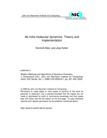
Ab Initio Molecular Dynamics TerminologyAb Initio Multiple Spawning DynamicsTodd J. MartínezDepartment of Chemistry & The Beckman InstituteUniversity of Illinois at ExtendedLagrangian?DynamicsDirect DynamicsDFTAb initioSemiempiricalAnyNoClassicalBOMDDFTAb initioAnyNoClassicalDFTPlane WaveYesClassicalDFT or SCFGaussianYesClassicalBorn-OppenheimerMolecular DynamicsCPMDCar-Parrinello MolecularDynamicsADMPAtom-Centered DensityMatrix PropagationElectronic Basis SetszPlane waves -e“Pulay” Termsikr– Natural for periodic systems– Hellman-Feynman Forces are exact– Very inefficient for nonperiodic systems (large empty spaces between periodicreplicas; in almost all cases, this empty space is filled with basis functions)– Obvious, well-defined convergence hierarchy zGaussian – e α r2 E ψ elec ( r ; R ) Hˆ elec ψ elec ( r ; R ) R R Hˆ elecψ elec ( r ; R ) ψ elec ( r ; R ) Rr“Hellmann-Feynman Force”r ψ elec ( r ; R ) ˆH elec ψ elec ( r ; R ) REmpty spacer ψ elec ( r ; R ) ψ elec ( r ; R ) Hˆ elec Rr“Pulay Force”– Periodicity is more difficult to incorporate (but not impossible, e.g. Crystal)– Generally atom-centered (“floating” Gaussians also possible)zElectrons like to be near nuclei!– Pulay terms in forces for atom-centered Gaussians– Convergence hierarchy more subtle, but now well-understood (Dunning)Pulay force apparently requires derivatives of electronic wavefunctions!Actually, often it does not, but it is always more expensive than HF ForceElectronic Excited StatesExtended Lagrangian TechniquezzWhat is it?– Electronic degrees of freedom are propagated under a new Lagrangian, instead ofusing the variational principle to determine them at each new geometryBenefits– Wavefunction does not need to be converged at each time stepzzzPhHC CH(CH3)2CC(CH3)2ONNMgNCO2CH3NREnergy transfer between ions and “fictitious” degrees of freedom is unphysical– Time step needs to be smaller than in BOMD – fictitious degrees of freedom arehigh-frequency relative to nucleiBottom line (according to TJM)– EL schemes have ½ time step to save 5 iterations/time step. Works out to a 2.5xspeed advantage in favor of EL– But need to be careful to maintain adiabatic separation of nuclei and electrons.– Both are reasonable and choice depends on tasteVisionHNOpsinEL expands dynamic range of frequencies to reduce SCF iterationsCH3CH3Energy Conversion“1” iteration vs. typical 10-15 iterations (apparently)But, good BOMD codes require 5 iter b/c geometry change in one time step is smallCH3hνPhPhDisadvantages– Need to ensure that the electronic coefficients are always “cold” and nuclei arealways “hot”zzPhChemical SynthesisCH3
Light-Driven Molecular DevicesMore Light-Driven DevicesLight Mechanical WorkhνFTour, Org. Lett. (2006)FHugel, et al, Science (2002)Yu, et al, Nature (2003)Other Applications Optical MemoryMolecular LogicLocal control of pH –“chemical circuits”Switch electron transport on and offDrug deliveryBalzani, Stoddart, PNAS (2006)Breakdown of Born-Oppenheimer ApproximationIncluding Quantum EffectszzzConical IntersectionsDegeneracy lifted in2-dimensional spaceAvoided CrossingsDegeneracy lifted inN-dimensional spaceClassical with “ad hoc corrections”– Not guaranteed to converge to the right answer – No well-defined nuclear wavefunctionMixed Quantum/Classical (See Iyengar Talk)– Based on time-dependent self-consistent field approximation– Not obvious that QM and CM are strictly compatible!Fully Quantum Mechanical– Approach is well-defined– But difficult (in fact, exponentially difficult in general case)– Basis set and path integral approacheszzCIs are the rule, not the exception: e.g., Michl, Yarkony, Robb, Nonadiabatic DynamicszEhrenfest Methodsrc&I i H IJ R cJ( )JAb initio Quantum DynamicsrrVave R cI*cJ VIJ R( )Feynman Path integrals– Imaginary time (quantum statistics) is easy– “Sign” problem in real time – progress, but still unsolvedBasis set– What kind of functions?– How to choose them?( )IJHamilton’s Eqns with Vave for R and PVave is unphysical asymptotically!Why? - Wavepacket splits into two partsand averaging becomes senseless Surface Hopping (Tully, Truhlar, many more )Avoid unphysical averagingStochastic “hops”No systematic hierarchyto improve approximations Ab Initio Quantum Dynamics “On-the-fly” solution of electronic andnuclear Schrödinger equations Multiple electronic states/Tunneling Need quantum nuclear dynamics Bond rearrangement Need to solve electronic Schrödinger equation Exact numerical solution of the nuclear Schrödinger equation is impractical for largesystems. Ab initio quantum chemistry is local Nuclear Schrödinger equation is global Not a problem in Car-Parrinello b/c Newtonian mechanics is local Further considerations: Need PESs for both ground and excited states. electronicψ electronicψJI Matrix elements which couple electronic states R Minimize the number of PESs evaluations b/c of extreme expense.Tailor the requirements of quantum dynamics to quantum chemistryand vice-versa!
Basis Set Approaches to Quantum Dynamicsδ ( x2 )Orthogonal basis of δ functionsδ ( x1 )Basis Set Approaches to Quantum Dynamicsψ ( x ) ciδ ( xi )χ2(x,t)χ1(x,t)it-dependent nonorthogonal basis setχ3(x,t)ci ψ ( xi )Determine ci(t) using FFT method, as describedby Batista yesterday For cognoscenti – the basis functions in the FFTmethod are actually sinc functionsψ ( x, t ) ci ( t ) χ i ( x, t )iNonorthogonal basisψ ( x, t ) ci ( t ) χi ( x ) χ ( x, 0 )ψ ( x, 0 ) dx c ( 0 ) χ ( x, 0 ) χ ( x, 0 ) dx c ( 0 )S ( 0 )j χ ( x )ψ ( x, 0 ) dx c ( 0 ) χ ( x ) χ ( x ) dx c ( 0 ) SjirrS 1ψ ( 0 ) c ( 0 )jiiiijzzzzzzzzaf a fz1 442 443Electronic statez Nuclear wavefunction on each electronic state is a product of 3Nzzfrozen Gaussian basis functions:a fa f χ Iiγ Ij t 3 NSemiclassical phaseρ 1af af( ( ))rRe χ Ij R, tρj ( Rρ ; Rρj t , Pρj t , α ρj )Position, momentum, widthCartesian degrees of freedom Classical evolution for R(t) and P(t). Variational principle for coefficients:()& iS 1 H iS& C H C CIII IIIIIIJJ Nuclear overlap matrixijNote this is NOT the time derivativeof the overlap matrix!Localization is good for scaling – analogy to local bases in quantum chemistryLocalization lends itself well to numerical approximations (e.g. integrals)Localization is needed for interface to electronic structure!Overcomplete if all p,q allowed – this will be good for us!Would a basis set of Gaussians with classical EOM be sufficient in principle?– Need to have classical energy width!– Otherwise, energy conservation will restrict allowed space– If no hidden conserved quantities and all energies are allowed, infinitebasis by this prescription will be overcomplete, hence the answer is YESPrinciple to PracticeII Wavefunction ansatz: Ψ R ; t C j t χ j R ; t Iχ Ij R; t e)Batista already showed us one way to get around this – adaptively expanding aGaussian basis set at each point in timeCould we make a good guess at the evolution of these basis functions?If we really believe that classical mechanics is usually sufficient, there shouldbe a way to take advantage of it!Why Gaussians (“coherent states”)?– Exhibit classical motion without deformation in harmonic potential– Minimum uncertainty states – as p/q localized as possible in QMzThe Full Multiple Spawning (FMS) MethodNuclear wavefunctionjiTime EvolutionIdeally, our basis set would be– Compact– Accurately describe the wavefunction at all times– Easily determined at any point in timeFixed basis sets (orthogonal and nonorthogonal)– Must span all Hilbert space which is sampled by the wavefunction frombeginning to end of simulation!– Recall Batista’s example of a Gaussian basis function evolving in aharmonic potential – it does not deform and its center follows classicalmechanics– With a fixed basis set, we must cover the entire configuration spaceaccessed– Even in 1D, the problem is much worse if wavefunction is unbound – forfree particle, we MUST have basis functions covering ALL spaceuniformlyI jii( S& ( t ) ) χ ( x, t ) t χ ( x, t ) dxIdeal Basis Seta fi& iS 1 H iS& C Insert ansatz into t-Dep Schrödinger Equation: C Set of ODE’s – integrate as discussed by Martynazji(jiidc iS 1HcInsert into t-Dep Schrödinger Equation:dtzirrS 1 ( 0 )ψ ( 0 ) c ( 0 )iHamiltonian matrixIn principle, we do not need to do anything special – just to have enough“trajectory basis functions”But who cares if the basis set prescription would be sufficient in principle?!Our computers have limited memory and we have limited lifespans Our basis set needs to be able to adapt to the problem!
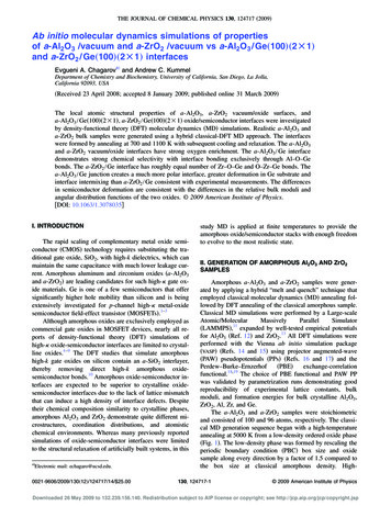
Adaptive Basis SetTime DiscretizationR(t)“Spawned” BasisFunctions Each basis function is “responsible” for a portion of the populationtransfer.Totalcrossingtime27654 crossingtime32108090 Basis set is small because crossing time is typically short. C(t) Effective non-adiabatic couplingNew Basis Functions added to augment classical mechanicsand accelerate convergencespawningthreshold100 110Time / fs120R Individual basisS functions T130Nonadiabatic Coupling RegionstimeTime DiscretizationCouplingCentral discretizationpoint should be chosenat maximum coupling,not midway in timeintervalMultiSpawn Æ Number ofdiscretization points per eventTimeOther discretization pointschosen to be equispaced in timeTime DiscretizationTime Discretization – Long EventsCSThreshCFThreshMaximum time for discretizationTimeEnd of “event”Start of “event”CouplingCouplingAvoid many smallspawning regionsTimeCSThresh CFThreshUsually chosen to be veryclose to each otherSpawn separately in each time intervalEach trajectory basis function canbe in “spawning” mode Æ In thiscase, it knows not to spawn againuntil a certain time is reached.
More Sophisticated Spawning SchemesWhere to Spawn? Want largest matrix element connecting new and old basis functions Demand Classical Energy Conservation – still have freedom“Constant Area” SpawningInvariant to time step; Under development0.01Spawning Energy for Spawned TrajectoriesEnergy for Spawned Trajectoriesk 10k 4Wigner view of SpawningxxWigner view of Spawningkk“position jump” type of behavior“momentum jump” type of behaviork 4k 10X
“Frustrated” SpawnsLinear Dependence and Matrix InversionWhen many gaussian basis functions are used, linear dependence may become anissueControlled by regularization– Singular value decomposition of Overlap Matrix– Singular values below a threshold are discarded– Norm conservation is affectedOverlap matrix does not have to be inverted. Solve by conjugate gradient (niceregularizing properties!):zEzEShellOnly FalsezSteepest Descent does not alwaysfind a solution within allottedtime. In this case, best solution isused iff EShellOnly False(Cost is N2 instead of N3, but sparsity makes it O(N)SteepestDescent lDiabatic vs Adiabatic RepresentationszzDiabatic– Smoother, therefore easier to integrate classical equations of motion fortrajectories– Couplings can be large – much spawning required– If diabatic model is purely quadratic, benefit from exact propagation whencouplings are small– Also, may be able to avoid integral approximations– Requires global information about PES – not suitable for ab initio MDAdiabatic– Nonadiabatic events are spatially/temporally localized – few spawningevents lasting for short timeAdiabatic– Classical mechanics is more nearly correctbecause electronic states are usuallyDiabaticindependentRunning A Simulation – FMS DynamicsFMS Dynamics– Widths need to be determined – these need to be tested for robustness –25% changes should not affect amount of population transfer– Need to determine appropriate values for CSThresh and CFThresh – thisneeds to be checked for every new molecule– Run several trajectories without spawning, monitor nonadiabatic coupling,choose thresholds low enough to capture all population transfer butotherwise as large as possiblezRunning a Simulation – AIMS DynamicszAb initio multiple spawning– Need to ensure that electronic structure method is accurate– This inolves iteration between AIMS and high-level electronic structure– Example with CASSCF – need to choose an active space and stateaveragingzzzzzz)& i H iS& C SC State ordering and S2/S1 gap at Franck-Condon pointPreliminary dynamics calculationCalculate CASPT2 PESs along CAS trajectories – demand consistencyMinimize snapshots from dynamics to find “attractor” minima or MECIsVerify energetics of these points withCASPT2 / MS-CASPT2CASIf inconsistent, dynamics results are discarded –continue search for active spaceCASPT2Multiple Spawning Two Diabatic Surfaces (A BC AB C collinear model) Triangles denote centroids of Gaussians – not all are populated! Linear dependence “prunes” number of Gaussians spawned “Back-spawning” is allowedVA BCVAB CInitial BasisSpawned Basis FunctionsFunctions Nonadiabatic Coupling Region
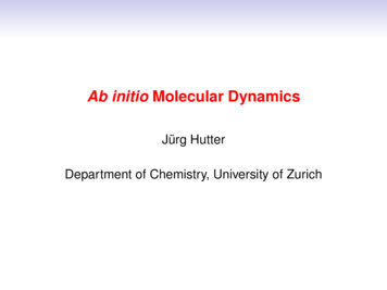
Initial ConditionsInitial ConditionspzSampling PointszzzqWigner distribution – only obtainable in practice within harmonicapproximationProblematic above v 0 because of negative regions; difficult to sampleNot appropriate for condensed phase because of many low frequencyvibrationsQuasiclassical Wigner – Use Wigner for chromophore and quasiclassical forremainder – for systems where chromophore/solvent decomposition is obviousOMaxI Æ if overlap between anytwo initial conditions OMaxI,one is rejected. Prevents excessivelinear dependence at t 0FirstGauss TrueGuarantees that the center of theWigner is first basis functionAbsorption and Resonance Raman SpectraCorrelation FunctionsTime-domain Formulation of Spectroscopy (Heller)1Electronic Absorption Spectrum: t I dtσ A FHω I IK Cω I φ i φ i et j expFH iωI Kz0.50.6 φ i μ eR j i ; φ i et j expGF iH ex t JI φ iHK00.4Resonance Raman Excitation Profiles:σ iR fFH IKω I C ′ω I ω 3sz 010.80.2 t I dtφ f φ i et j expHF iωI K2-0.50-1001000 2000 3000 4000 5000 6000 7000 80001000 2000 3000 4000 5000 6000 7000 8000Time / atuTime / atu Anharmonicity and Duschinsky rotation included Coordinate dependence of transition dipole can be includedCorrelation Function Æ SpectrumConvergence10.81 BFxn10 BFxns0.60.420 BFxns10 BFxns0.2001000 2000 3000 4000 5000 6000 7000 8000Time / atu-1.5-1-0.500.511.5Energy / eV-1-0.50Energy / eV0.51-1-0.50Energy / eVEthylene V State, Vibronic Coupling Model0.51
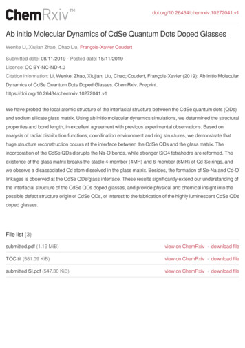
Pyrazine Electronic Absorption SpectraS1Effect of Nonadiabaticity on SpectrumS2NMCTDHNonadiabaticN Structureless S2 spectrum implying fast S2 S1 internal conversion 3D/4D/24D vibronic coupling (Domcke/Cederbaum/Meyer/Koppel)H0 C(t) limited to 150fs – stillleads to significant structurew/o nonadiabaticity MCTDH for comparisonAdiabatic150fs1 2 ωi ( Q2 Qi2 )2 ii E H κ(1)Q κ(1)Q λQ10aH 1 0 1 1 6a 6a λQ10aE1 H0 κ1(2)Q1 κ(2)6a Q6a Results for Electronic SpectraPyrazine:3 dimensional modelPyrazine:4 dimensional modelDependence on Spawning ThresholdPyrazine:24 dimensionsλ 2.5 Prespawning used in all of these calculations Final number of basis functions ranges from 100-900 Somewhat better agreement from IVR methods w/ 106 trajectories Small thresholds required to reproduce detailed structure Smooth convergence observed Fewer basis functions may suffice in adiabatic representationAccuracy of FMS Method: The Spin Boson ModelSaddle-Point ApproximationsIntegrals which are difficult to evaluate in AIMS are treated with saddle pointapproximation:χ VIJ χIiJj χ χIiJjVIJ ( R )zTwo level system linearly coupled to a Harmonic bath:zIn the diabatic representation:H H S H B H S BH ϕk 1,2w/SPAzw/o SPAMinimal effect on spectrumkhk ϕk { ϕ1 Δ ϕ2 c.c.}hk h0 C j X jCentroid of Product Gaussian(Higher order variants possible,but require Hessian)00 Large spawning thresholds get basic envelope correctThoss, Miller and Stock, JCP (2000)zλ 20.0λ 5.00zzzωj;h0 -- vibrational frequencyj of the jth oscillator-- dimensionless linear coupling of the jth oscillator-- electronic coupling-- dimensionless position and momentum1 ω j ( Pj2 X 2j )2 jCjΔX j , PjIn the form of Domcke-Cederbaum-Koppel vibronic coupling modelsOften used as a model for conical intersection problems
The Spin Boson ModelzBath properties are determined by the spectral density:J (ω ) zExtended Coupling RegionsThe case of an Ohmic bath:J (ω ) π2π2z C δ (ω ω )2jzjzj 2 C j Δω J (ω j ) π α e ω ωc12Adaptive expansion is tailored to time/space-local breakdowns of the BornOppenheimer approximationWhat about cases where the BOA breaks down completely?Continuous spawning – ensure that basis functions always have “partners” on otherelectronic states when they are coupled. Why is this even practical? PESs tend to benearly parallel in extended coupling regions!Exact Results:z 400 dimensional model– C. H. Mak and D. Chandler, Phys. Rev. A 44, 2352 (1991)– D. E. Makarov and N. Makri, Chem. Phys. Lett. 221, 482 (1994)– R. Egger and C. H. Mak, Phys. Rev. B 50, 15210 (1994)z 4 dimensional model– G. Stock, J. Chem. Phys. 103, 1561 (1995)– Multiconfigurational Time-Dependent Hartree (MCTDH)zManthe, Meyer, Cederbaum Chem Phys Lett 165, 163 (1990)12.0 -10.0 -8.0 -6.0 -4.0 -2.0Spin Boson Tests – 4 DOF0.02.04.06.08.0 10.0 12.0Spin Boson Tests – 400 DOFSurface HoppingFMS-CSNumerically ExactSurface-HoppingEhrenfestIn high dimensionality and finite T, convergence is actually faster –basis function separation is physically correct.(See early work by Neria & Nitzan, Rossky, Bittner)Multiple SpawningIndependent First-Generation Approximationψ ciψ iIFGTime FMS is a hierarchy of methods Dynamics on a single electronic state coupled frozen Gaussians (Heller,Metiu) Useful Approximations in Ab Initio Dynamics Independent First Generation Approximation Different initial Gaussian wavepackets are uncoupled Includes coherences between basis function and its “children” Neglects coherence between initial basis functions Saddle-Point Approximation for Integrals Use locality of Gaussians to evaluate integrals using local information χi R f (R)χ j R dR f Rc χi R χ j R dR Centroid of χiχjiOˆψ ci*ci OˆiψiRun 1Run 2
Saddle-Point ApproximationsEOM-CCSD Spectra for EthyleneR3s and V spectra shifted to large basisMRSDCI vertical excitation energiesR3sf 0.15AIMS-EOM-CCSD χi R f (R)χ j R dR χi R χ j R f ( R ) ( R R ) R fc ( R Rc )cRc2 2 f R 2Rc L dR f ( R ) χi R χ j R c Expt Vf 0.38 Taylor expansion of potential around maximum of product First-order term requires gradient at maximum of product Second-order term can be included if Hessian of potential availablePhotochemistry /Photophysics of EthyleneAIMS Excited State Dynamics of Ethylene Prototype for cis-trans isomerization Conventional Picture:hνφ50 fs0 fs110 fs150 fscis Δq / electrons1transφ One-dimensional nature - emphasizing torsion Chemistry and Isomerization occur on S0 Experimental Photoproducts: cis-trans isomers, HC CH, H2, H Excited State Lifetime from Absorption Spectrum: 50 fs No fluorescenceEthylene Dynamics Overview170 fsΔq qel ( CH 2 )0 .8Left qel ( CH 2 )Right0 .60 .40 00300Time / fsDo Conical Intersections Matter?0.16Population 100.150.20Minimum Energy Gap (eV)Charge Transfer State Critical to S1 DecayTorsion alone is insufficient – in contrastto textbook pictureRegions near intersections dominate nonadiabatic events350350
Do Minimal Energy Conical Intersections Matter?q(C2H3leftcharge) – q(C/ 2qHe 3right)0.16FC Point0.140.12PopulationPhotoinduced cis-trans Isomerization - 175100time / fs0.00012345Twist Angle / degMinimal energy point along seammay have little significance!Still useful in cartoon pictures ofmechanisms0100175Central150Energy above MECI (eV)175C3C2H2C1H1100Again, charge transfer stateplays key me / fsExcited State Intramolecular Proton TransferMethyl Salicylate Energy DiagramFCS1 ketoS1 6-0.48HHOOCHOhν CCHOCHCC1.78HHHSA2-CASPT(2/2)No H/D isotope effect!?Experiments: Lochbruner, Stolow, Riedle, Zewail Time / psLochbrunner,JCP (2001)H-Atom Transfer in Methyl SalicylateExperimentIsotope Effects in MS ESIPTS0 KetoS1 EnolH-Atom Transfer TimeExpt: 60 10 fs (Herek)AIMS: 50 fsSA-2-CAS(2/2)-PT2AIMS DynamicsCASPT2 Gradients:Celani and Werner, JCP 119 5044 (2003)No significant isotope effect!
Bond Alternation “Gates” H-Atom MotionWavepacket Dynamics on S1Reduced densitiesdetermined byMonte Carlo integrationusing FMS wavefunctionS0 KetoAH-DHrrrrρ ( r ) dxψ * ( x )ψ ( x ) δ ( r ( x ) r )C7-OaS1 EnolTime/Energy-Resolved Fluorescence SpectraIntersections from Semiempirical CASCIzzzzSemiempirical analog of state-averaged multi-reference ab initio methodsGood agreement with ab initio CASSCF results– Qualitative intersection geometries– Coordinates which lift electronic degeneracyBUT, energetics are qualitatively incorrectSuggests feasibility of reparameterizationMS-HMS-DExpAIMSComparison of intersection geometries and modes which lift degeneracy inretinal protonated Schiff base analogExpt: Herek, Pederesen, Banares, and Zewail,JCP 97 9046 (1992)RPSB Analog ReparameterizationzzMultireference semiempirical model – Fractional Occ MO*CAS(6/6)-CICombine with QM/MM model to represent solventAb initio data included in reparameterization– SA-2-CAS(10/10)/6-31G*– S0/S1 excitation energy at S0 minimum– Relative energies of MECIs for 11-12 and 13-14 11S00.504013.53.5Energy / eVzRPSB Analog – RPSE-CAS(6/6)6080100C C1112120140Twist Angle160S10.51800406080C C1112100120140160Torsion Angle / Degrees180
RPSB Analog – RPSE-CAS(6/6)Energy / 4080C C910120160Hˆ TOT Hˆ QM Hˆ QM / MM Hˆ MM13.50.5QM/MM Semiempirical FOMO-CAS CI σ 12 σ 6 ZZ ZHˆ QM / MM m α m 4ε α m α m α m Rim rimα m Rα mα m Rα m α m RPSEQM electrons / nucleiMM nucleiS10.500Twist Angle4080120160Solvated GFP ChromophoreConical IntersectionC9 C10 Twist AngleComparisons for torsion around bonds not included in reparameterizationRPSB Isomerization QY / LifetimePopulation ratio1RPSB / MeOH FluorescenceQM/MM Model80 OPLS/AA MeOHMeOH, S10.8all-trans, S0Gas Phase, S10.60.4Isomerized, S00.200100020003000Tim e/fs40005000Isomerization QY: 13%-20% (Expt)24% (Theory, MeOH)38% (Theory, Isolated)Lifetime: 2-12 ps (Expt)Photoproduct branching: 1:6:4 (13-cis:11-cis:9-cis) MeOH1:3:2 IsolationKandori & Sasabe, CPL 1993τ1 35fsτ2 2.5psτ1 90fsτ2 3-4psIsolated RPSB FluorescenceRPSB Isomerization BarrierC-backbone fixed2.52eV1.5RPSB, isolated1RPSB/MeOH0.5Much shorter lifetime in isolationDominant product 11-cis in bothMeOH and gas phaseτ 205fs090110130150170C11 C12 torsion angleNo barrier in gas phaseWhat causes barrier in solution?
RPSB Free Energy Surface on S1Origin of RPSB/MeOH Isomerization BarrierFree Energy Barrier at θ 120 C11 C12C11 C120.0060.0080.00610.0201.351.45X DataBond 50charge0.010rn X Dati ataonrZ 1.40140Torsio Y Da 100n Antagle 40120.0TorsionY DataAngle θ16080.000.006180Need free energy surfaces to understand behavior in solution!0.2qright - Isolatedqright - MeOH090100110120130140150160170180C11 C12 torsion angleG (θ , r ) kT ln P (θ , r )Conical intersection TopographyReparameterized Semiempirical CASCICASSCF“Peaked”“Sloped”RPSECASPT2Green Fluorescent ProteinRPSE fit to EOM-CCSD in FC regionToniolo, TJM and coworkers: JPC 106A 4679 (2002); JPC 107A 3822 (2003);Chem Phys 304 133 (2004); Far. Disc. 127 149 (2004)Reparameterized SE S1 Dynamics100fs to reach twisted geometryNo quenching at 250fsInitial dynamics dominated by H motionReparameterized SE QM/MM S1 Dynamics60fs to reach twisted geometryQuenching begins at 60fsSolvent stabilizes conical intersectionInitial dynamics similar to gas phase150 TIP3P Water Molecules
Solvent Effects on Conical IntersectionsGFP neutral chromophore lifetimeIntersection becomesabsolute minimum!5Energy / eV4VacuumVacuum3Hydrated21Water0S0 minimumS1 minimumI-Twisted MECINeutral in the ProteinSolvent Effect on Topography1.0ψ covalentS1ψ CTsolvatedWhen one state ispreferentially stabilized,intersections become1) Peaked2) Absolute minimaPopulation0.8ψ CTS00.60.40.2S20.00200400600800100012001400Time, fs180160Faster decay than in vacuum Angle, 00Time, fsAnion in the Protein1.0Population0.8Can tunneling be included in multiple spawning? Trivial case: Tunneling in a multi-electronic state framework But we do not want to include more electronic states!S10.60.4S00.2S20.00200400Tunneling via Multiple Spawning Dynamics600800100012001400Time, fsSingle-Surface Spawning Label atoms which may tunnel Label sites where atoms may tunnel Spawn basis functions where neededsingle stateAngles, degrees80Spawned Basis FunctionIP60402000200400600800Tims, fs100012001400multi-state
Single-Surface Spawning ResultsSingle-Surface Spawning Test 2-D Model for Proton Transfer1f (s) V ( s, Q ) V0 ( s ) 12 mω 2 Q mω 2 2FHS FH t IK ψ GFH 0JIK ψ FH t IKQuantumFMSIKReG S FH t IK JV0 ( s ) 21 as 2 14 bs 4Average .5FHIKImG S FH t IK Jf ( s ) cs 2f ( s ) cs0-1Single-Surface Spawning Spectrum0200400600Time / fs800105013501000Frequency / cm-1Q uantu mFMS950850115080011000.0020.004 0.006 0.008C oupling / a. u.850v 18001050Q750C oupling / a. u. Agreement of Tunneling Splitting isbetter than absolute frequencies0.006100-10.004Tunneling Splitting / cmFrequency / cm-111500.0 0280Q uantumFMS604020000.0020.004C oupling / a. u.10500.01Single-Surface Spawning Wavefunction900012501200v 0Single-Surface Spawning for Linear Coupling13009000v 0800 1000 120010007501100600Single-Surface Spawning for Quadratic CouplingTunneling SplittingFMS:91.89 cm-1Quantum: 91.90 cm-1QuantumFMS400Note agreement for S(t) This requires correctphase interference!-0.5 15 Basis Functions to represent Initial State Wavefunction propagated for up to 4 ps Up to 30 final basis functions (15 spawned)200Time / fs00.006QuantumFMSsv 1
AcknowledgmentsJiahaoChenAaronVirshupJoshua CoeBen LevineAlexisThompsonCollaboratorsH.-J. Werner – FMS-MolProJ. J. P. Stewart – FMS-MOPACM. Persico – FMS-MOPACA. StolowC. BardeenJ. MooreK. SchultenFunded ongChaehyukKrissie LamotheKoCHE, BESDMR, CISE
Ab initio Quantum Dynamics. Basis Set Approaches to Quantum Dynamics δ(x1) δ(x2) Orthogonal basis of δfunctions ( ) ii i ii x cx cx ψ δ ψ Determine ci(t) using FFT method, as described by Batista yesterday For cognoscenti - the basis functions in the FFT method are actually sinc functions Nonorthogonal basis ()() ( ) () () 1 (),,0 0 0 00 ii i j ij i i ji ii xt c t x x xdx .