Transcription
Ab initio Molecular DynamicsJürg HutterDepartment of Chemistry, University of Zurich
Overview Equations of motion and Integrators General Lagrangian for AIMD Car–Parrinello MD and Born–Oppenheimer MD ab initio Langevin MD Stability and efficiency Thermostats External Drivers
Equations of Motion (EOM)Newton’s EOM for a set of classical point particles in apotential.MI R̈ I dV (R)dR IThese EOM generate for a given number of particles N in avolume V the micro canonical ensemble (NVE ensemble).The total energy E is a constant of motion!
Total EnergyTotal Energy Kinetic energy Potential energyKinetic energy T (Ṙ) NXMII 12Ṙ2Potential energy V (R)We will use the total energy as an indicator for the numericalaccuracy of simulations.
Lagrange Equation Ld L dt Ṙ RwithL(R, Ṙ) T (Ṙ) V (R)Equivalent to Newton’s EOM in Cartesian coordinates, but ismore general and flexible. Extended systems Constraints
Integration of EOMDiscretization of timeR(t) R(t τ ) R(t 2τ ) · · · R(t mτ )V (t) V (t τ ) V (t 2τ ) · · · V (t mτ ) Efficiency: minimal number of force evaluations, minimalnumber of stored quantities Stability: minimal drift in constant of motion (energy) Accuracy: minimal distance to exact trajectory
Sources of Errors Type of integratorpredictor-corrector, time-reversible, symplectic Time step τshort time accuracy measured as O(τ n ) Consistency of forces and energye.g. cutoffs leading to non-smooth energy surfaces Accuracy of forcese.g. convergence of iterative force calculations (SCF,constraints)
Velocity Verlet IntegratorR(t τ ) R(t) τ V (t) V (t τ ) V (t) τ2f (t)2Mτ[f (t) f (t τ )2M Efficiency: 1 force evaluation, 3 storage vectors Stability: time reversible Accuracy: O(τ 2 ) Simple adaptation for constraints (shake, rattle, roll) Simple adaptation for multiple time steps and thermostats
Test on Required Accuracy of ForcesClassical Force Field Calculations, 64 molecules, 330 KTIP3P (flexible), SPME (α 0.44, GMAX 25),
Stability: Accuracy of ForcesStdev. fHartree/BohrStdev. �10 1010 0810 0710 0610 0510 04DriftµHartree/ns -0.140.01-0.10-0.6315.211599.31
Born–Oppenheimer MD: The Easy WaydV (R)EOMdR IV (R) min [EKS ({Φ(r )}; R) const.] Kohn–Sham BO potentialMI R̈ I ΦForcesd minΦ EKS ({Φ(r )}; R)dR EKS const. X (EKS const.) Φi R R Φi Ri {z}fKS (R) 0
Computational Details System 64 water molecules density 1gcm 3 Temperature 330K Timestep 0.5fs DFT Calculations GPW, TZV2P basis (2560 bsf), PBE functional Cutoff 280 Rydberg, default 10 12 OT-DIIS, Preconditioner FULL SINGLE INVERSE Reference trajectory (1ps), SCF 10 10
Stability in BOMDUnbiased initial guess; Φ(t) Φ0 (R(t)) SCFMAE EKSHartreeMAE fHartree/BohrDriftKelvin/ns10 0810 0710 0610 0510 041.2 · 10 119.5 · 10 106.9 · 10 087.4 · 10 063.3 · 10 045.1 · 10 095.6 · 10 084.8 · 10 075.6 · 10 065.9 · 10 050.00.10.42.350.0Consistent with results from classical MDNote accuracy of forces!
Efficiency: Initial Guess of Wavefunction4th order Gear predictor (PS extrapolation in CP2K)Method SCFIterationsDrift (Kelvin/ns)Guess10 0614.380.4Gear(4)10 076.475.7Gear(4)10 065.2211.8Gear(4)10 054.6086.8What is the problem?Time reversibility has been broken!
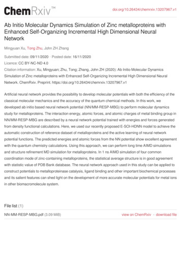
Generalized LagrangianL(q, q̇, x, ẋ) 11M q̇2 µẋ2 E(q, y) k µG(kx yk)22y F (q, x)wavefunction optimizationG(kx yk)wavefunction retention potentialEquations of motion E E F G F kµ q y q y q G G F E Fµẍ kµ y x x y xM q̈ Extension of Niklasson Lagrangian, PRL 100 123004 (2008)
Dynamical System
Car–Parrinello Molecular Dynamicsy x G(kx yk) 0LagrangianL(q, q̇, x, ẋ) 11M q̇2 µẋ2 E(q, x)22Equations of motion E q Eµẍ xM q̈
Properties of CPMD Accuracy: MediumDistance from BO surface controlled by mass µRequires renormalization of dynamic quantities (e.g.vibrational spectra) Stability: ExcellentAll forces can be calculated to machine precision easily Efficiency: GoodEfficiency is strongly system dependent (electronic gap)Requires many nuclear gradient calculationsNot implemented in CP2K!
BOMDy Minx E(q, x) and µ 0Lagrangian1M q̇2 E(q, y)21L(x, ẋ) ẋ2 kG(kx yk)2L(q, q̇) Equations of motion M q̈ E qdecoupled equations ẍ k G x
BOMD with Incomplete SCF Convergencey F (q, x) Minx E(q, x)and µ 0Equations of motion E F E q y q G G F ẍ k x y xM q̈ SCF Error: Neglect of force terms E F y qand G F y x .EOM are coupled through terms neglected!
ASPC IntegratorIntegration of electronic DOF (x) has to be accurate: good wavefunction guess gives improvedefficiency stable: do not destroy time-reversibility of nuclear trajectoryASPC: Always Stable Predictor Corrector J. Kolafa, J. Comput Chem. 25: 335–342 (2004) ASPC(k): time-reversible to order 2k 1
Orthogonality ConstraintWavefunction extrapolation for non-orthogonal basis setsCinit KXBj 1 Ct jτ CTt jτ St jτ Ct τ{z} j 0PSCoefficients Bi are given by ASPC algorithmx Cinity[t] CtS overlap matrixJ. VandeVondele et al. Comp. Phys. Comm. 167: 103–128 (2005)
Importance of Time-ReversibilityMethod SCFIterationsDrift (Kelvin/ns)Guess10 0614.380.4ASPC(3)10 065.010.2ASPC(3)10 053.024.5Gear(4)10 076.475.7Gear(4)10 065.2211.8Gear(4)10 054.6086.8
Efficiency and DriftMethod SCFIterationsDrift (Kelvin/ns)Guess10 0614.380.4ASPC(4)10 065.010.2ASPC(4)10 053.024.5ASPC(4)10 041.621742.4ASPC(4)10 021.0321733.2
Efficiency and DriftMethod SCFIterationsDrift (Kelvin/ns)ASPC(4)10 041.621742.4ASPC(5)10 041.631094.0ASPC(6)10 041.79397.4ASPC(7)10 041.97445.8ASPC(8)10 042.0624.1
Langevin BOMDStarting point: BOMD with ASPC(k) extrapolationAnalysis of forcesfBO (R) fHF (R) fPulay (R) fnsc (R){z} f (R) fBO : correct BO force fHF : Hellmann–Feynman force fPulay : Pulay force fnsc : non-self consistency error force f : approximate BO force
Forces in Approximate BOMDApproximate fnsc byf̃nsc Zdr Vxc (ρi ) ρi ρ VH ( ρ) I ρiwith ρ ρo ρi , ρo final (output) density, ρi initial (predicted)density.Now assumef (R) f̃nsc (R) fBO (R) γD Ṙwhere γD is a constant friction parameter.
Langevin EOMM R̈ fBO (R) (γD γL )Ṙ Θwith Θ a Gaussian random noise term andhΘ(0)Θ(t)i 6(γD γL )MkB T δ(t)Given temperature T determines γD2kB3 hM Ṙ iand an arbitrary γL this
Langevin BOMD2nd Generation Car–Parrinello (SGCP)T. D. Kühne et al., Phys. Rev. Lett. 98 066441 (2007) single SCF step plus force correction neededextremely efficient for systems with slow SCF convergence γD is small: correct statistics and dynamics difficult to stabilize in complex systems
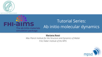
SGCP: ExamplesT. Musso et al. Eur. Phys. J. B, 91 148 (2018)Analysis of Force ErrorsLiquid Silicon at 3000 K
SGCP: Nanomeshh-BN on Rh(111)
SGCP: Force Errors
SGCP: h-BN on Rh(111)Comparision of MD Results
SGCP: h-BN on Rh(111)Performance
Micro-Canonical Ensemble System variables: N, V, E Microstate definition: Γ {r N , p N } Energy H(Γ) Ppi2i 2mi U(r N ) All states have the same weight δ(H(Γ) E) PartitionfunctionΩ(N, V , E) XΓ1 1δ(H(Γ) E) N h3NZdr N dpN δ(H(Γ) E)
Molecular Dynamics Fixed number of particles: N Fixed volume: V Periodic boundary condition to avoid surface effects Total energyE(t) X mii2ṙi2 (t) U(r (t))
Constant of Motion: EX dU(r )dE(t) X mi 2ṙi r̈i ṙidt2driiidU(r ) mi r̈iFi driXXFiĖ mi ṙi ( Fi )ṙimiiiX (ṙi Fi ṙi Fi )i 0The energy is conserved. MD samples correct microstates.
Definition of TemperatureInstantaneous temperatureT (t) 2 1Xmi ṙi2 (t)3NkB 2iTemperatureT hT (t)i
Equipartition TheoremThe equipartition theorem is a general formula that relates thetemperature of a system with its average energies. For asystem described by the Hamiltonian (energy function) H(r , ṙ ) H Hri pi δij kB T rj pjFor an ideal gashHi hHkin i 3kB T2
Canonical Ensemble System variables: N, V, T Closed system exchanging energy with a heat bath attemperature T.How to simulate on a computer? We can directly manipulate velocities (temperature). No extended heat bath needed. Molecular dynamics with periodic boundary conditions, butmanipulate ṙi during the integration.
Control of velocities/temperature Differential control: the temperature is fixed to thepredescribed value and no fluctuations occur. Proportional control: velocities are corrected at eachintegration step through a coupling constant towards theprescribed temperature. The coupling constant determinesthe strength of the fluctuations around hT i. Integral control: the Hamiltonian is extended and variablesare introduced wich reflect the effect of an external systemwhich fix the temperature. Time evolution is derived fromthe extended Hamiltonian. Stochastic control: position and velocities are propagatedaccording to modified equations of motion with friction andstochastic forces. The final equations give the correctmean value of the temperature.
NVEΓ {rN , pN }H(Γ) microstateNX1pi U(rN )2miconst.i 1All accessible microstates are equally probableWNVE (Γ) δ(H(Γ) E )statistical weightDistribution of microstatesΩNVE XΓδ(H(Γ) E ) 1 1N! h3NZdrN pN δ(H(Γ) E )5/1
Canonical Ensemble (NVT)Microstates follow the Boltzmann’s distribution H(rN , pN )WNVT (Γ) exp kB TCanonical partition function: describes the statistical properties ZXH(Γ)1H(rN , pN )NNQNVT exp drdpexp kB TN!h3NkB TΓProbability distributionP(Γ) WNVT (Γ)QNVTand the expectation value of the total energy is (β 1/kB T )( )X ln QNVT1H(Γ)hE i H(Γ) exp βQNVTkB TΓ
Velocity RescalingAt t and temperature T (t) all velocities are multiplied by λ T NNi 1i 11 X 2 mi (λvi )21 X 2 mi vi2 (λ2 1)T (t)23 NkB23 NkBTo control the temperatureλ pT0 /T (t) Easy to implement Sampling does not correspond to any ensemble Not recommended for production MD Good for equilibration Not time-reversible, not deterministic24 / 1
Velocity rescalingPerform one (or more) MD stepsCompute the instantanous kinetic energyRescale the velocities by a factor25 / 1
Jumps rescalingby Rescaling (II)Velocity20! 1K1510500204020t6080100! 10K15105002040t608010026 / 1Pisa, Scuola Normale – p. 25/73
Berendsen ThermostatWeak couplingto a heatbath: temperature correctionBerendsenThermostatdT (t)1 (Tbath T (t))Another populardtvelocityτ scaling thermostat is that of Berendsen. Here,the scaling is given byτ coupling parameter: larger τ weaker coupling!"f the1 desiredTmd temperatureExponential decay of the systemdvtowardsdt m 2τT (t) 1 v(13)δt T (Tbath T (t))τ of the thermostat. It describes the strength ofτ is called the ‘rise time’the coupling of the system to a hypothetical heat bath.The larger τ , the weakerthe coupling, i.e., theτ , thermostatis inactivelongerit takes to achievetoo small τ , unrealisticallyfluctuationsa given Tmdlowfromthe curT (t):τ δt, standardrentrescalingTSame problems as velocity rescalingTime27 / 1Simulation of Biomolecules –
Like a frictionContinuous formulation of the velocity rescalingṗi fi ζpi P 2 1/2piδt i mi 1 (1 ζδt) 1 τNkB T Friction positive whenK NkB Tthermostat/2, cooling. (III)Berendsen20! 1K1510500204020t60100! 1015K80105002040t6080100
Langevin ThermostatRandom forces due to impacts exerted by molecules in the environment:irregular motion and friction. At each step all vi are corrected by arandom force and a friction termmr̈i U mΓṙi Wi (t) riFrictional force and random motion are related, i.e.fluctuation–dissipation theorem is satisfiedhWi (t), Wj (t 0 )i δij δ(t t 0 )6mΓkB TGaussian distribution with infinitely short correlation time (great numberof collisions)Transition probability X pi P P U P 2P pi P mi D 2 Γ tmi ri ri pi pi pii
Stochastic BehaviorThe canonical distribution is then recovered as1 X mp2ilim P C exp { U(rN )}t kB T2i!and friction and diffusion are relatedD ΓkB TmLocal thermostat: noise term depends on the particle Samples from canonical ensemble and ergodic. Allows larger time steps compared to non-stochastic thermostats. Momentum transfer is destroyed, i.e., no diffusion coefficients.34 / 1
Nose ThermostatHeat bath integral part of the system: s, ṡ, and Q (coupling)L X ms 2 ṙ2ii21 U(rN ) Q ṡ 2 gkB T ln s2The conjugate momenta in the extended system arepi L mi s 2 ṙi ṙips L Q ṡ ṡwhere the auxiliary variable is a time-scaling parameterdt 0 sdtp0i p/sreal system momentumMicrocanonical ensemble in the extended system: for g 3N 1canonical ensemble for the real system38 / 1
Nose–HooverUsing only differentiation in real time t 0 :ṙi ṗi ξ ṡsHNose pimi U ξpi ri1 X p2iQimi 1 ds dt 0gβξ sps /Q!d ln s ξdtX piξ2Qln s U(rN ) g2mi2βconservedi39 / 1
Friction CoefficientDefine the relaxation time asνT p3NkB T /Qdynamics of friction coefficient by (feed-back mechanism) P 2 piim2 Ti ξ νT2 1 νT 13NkB TTToo large Q: canonical distribution after long simulationToo small Q: high-frequency T oscillations
Ergodicity ProblemsMicrocanonicAndersenNose-HooverrrrvNVE: closed loop, constant energy shellAndersen: points corresponding to a Gaussian velocity distributionNose–Hoover: band trajectory determined by the initial conditionsNot sufficiently chaotic to sample all phase-space; trapped in a subspace41 / 1
Nose–Hoover ChainErgodicity is improved by thermostatting the thermostat variable: MNose–Hoover thermostatsHNHC ṙi ṗi ξ 1 ξ j ξ M pimi U ξ1 pi ri!1 X p2 giQ1imi β ξi ξ2 12Qj 1 ξj 1 kB T ξj ξj 1Qj 12 kB TQM 1 ξM 1QMMX piX Qj ξj2X U(rN ) gkB Ts1 kB Tsj2mi2ijj 242 / 1
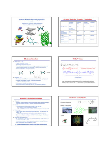
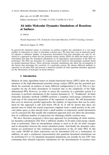
Thermostats Comparison600velocityvelocity position02468velocityNose-Hoover chain2000150010005000position24Time [ps]6843 / 1
ThermostatsTableThermostattabletunecont.Velocity rescalingL/Gcorrect ergodic cons. q. Nosé-HooverchainsXXL/GXLangevinXXLStochastic R**XXXCSVR*use “LENGTH 1”**use “MASSIVE”44 / 1
Other EnsemblesN, V, Emicrocanonicalinner energy UN, V, TcanonicalHelmholtz free energy FN, P, Hisobaric-isoenthalpicF U TSenthalpy HH U pVN, P, Tisobaric-isothermalGibbs free energy GG U TS pV H TS
How to simulate an isobaric ensemble? We can manipulate the volume of the system. This emulates an external piston used to keep thepressure constant. Instantaneous pressure p(t) fluctuates, forces on thecontainer Averaging p(t) gives the observable internal pressure.
Pressure: Virial TheoremFrom equipartition theorem* X p21X U(r )ihHkin i ri2mi2 riiiThe total potential U(r ) is coming from in internal potentialVint (r ) and and a wall potential W (r ).ZZX W (r )ri p df · r p dV (divr ) 3pV riiThe virial theorem is thenX V (r )3pV 2hHkin i ri rii
Isobaric-Isoenthalpic EnsembleThe system exchange work with an external surface: Ω is a variableCubic box 100Ω31h 0 Ω30 100 Ω3Scaled coordinatesri Ω1/3 siLagrangian in terms of scaled coordinatesL 21Xmi Ω 3 ṡ2i U(sN , Ω)2iExternal applied pressure P P Ωwork on the system to balance P: the internal pressure fluctuates46 / 1
BarostatCorrect the internal pressure by scaling the voluem, i.e. the inter-particledistancesThe system is coupled to a barostatIsobaric-Isoenthalpic ensemble NPHP(rN , pN , Ω) δ(C K(pN ) U(rN , Ω) ΠΩ)where Π is the internal pressureIsobaric-Isothermal ensemble NPT K(pN ) U(rN , Ω) ΠΩNNP(r , p , Ω) exp kB T47 / 1
Berendsen BarostatDeviation from desired pressuredP(t)P0 P(t) dtτPτP relaxation timeRescale volume by η the volume, η 1/3 coordinatesη(t) 1 δtγ(P0 P(t))τPγ is the compressibility.Asotropic or anisotropic, τP strength of coupling,not correct ensemble distribution
Andersen BarostatAssociate a kinetic energy to the variable volumeL 21X1mi Ω 3 ṡ2i W Ω̇2 U(sN , Ω) PΩ22iThe coupling mimics the action of a piston of mass W (strength ofcoupling)Equations of motions̈i 1W Ω̈ 3ΩΩ23Xi1 U2 Ω̇ si23Ωmi Ω 3 simi ṡ2i Xi Usi si! P Pint PFeedback loop to adjust the simulation volume: internal pressurefluctuates around the external pressure49 / 1
Correct DistributionConserved Hamiltonian of the 6N 2 dimensional systemH Π21 X π 2i U(sN , Ω) PΩ2 22Wmi Ω 3ilow W will result in rapid box size oscillationslarge W slow adjustmen of the volumePartition function ZZZZΠ2 (N, P, H) dΩ dΠ dπ N sN δ H H2Wtrajectories consistent with the NPH ensembleThe combination with one of the constant temperature methods allowsthe simulation in the NPT ensemble.50 / 1
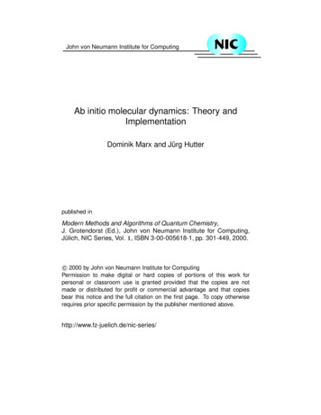
Experiments with barostats ExperExperiment with barostatand thermostatEqEquilibration with BerendsenCons. [kJ/mol]-1000Experiments with barostatsExperiments with barostats-1100-1200-1300-1400Equilibration withBerendsenBerendsenThermostat and Barostat-1100τT 0.1-1200τP 1, 2, 4, 8Cons. [kJ/mol]Cons. [kJ/mol]-1000-13001.5τT 0.11τP 1, 2, 4, 80.53V [A ]1200011000τP 1, 2, 4, 861250054120003211500111000001250011500τT 0.110-3051300013000120001.5-300 0.50130003V [A ],8-2953P [katm]V [A ]P [katm]-14002P [katm]2 Nose--HooverEquilibrationwith Nosé-HooverThermostat and Barostat510time (ps)201511000Pisa, Scuola Normale – p100000510time (ps)1520Pisa, Scuola Normale – p. 64/730510time (ps)1520Pisa, Scuola Normale – p. 65/7351 / 1
Multiple Time Step Method (r-RESPA)M.E. Tuckerman et al. JCP, 97 1990 (1992)Equation of motionṙ iL pmṗ Ffast FslowLiouville operator p Ffast iLref iLslow Fslowm r p pIntegratorx(δt) exp(iLδt)x(0) exp(iLslow δt/2) [exp(iLref δt)]n exp(iLslow δt/2) O(δt 3 )
MTS in CP2K Two FORCE EVAL sections defining methods Example DFT with hybrid functionalsFref FGGAFslow Fhybrid
PLUMED: MD Driver and Enhanced Sampling Definition of many Collective Variables (CV) Analysis features for MD and MetaDynamics Bias methods for enhanced sampling MD Logarithmic Mean Force Dynamics Method Experiment Directed Simulation Methods
i-Pi: External MD DriverKapil et al., Comp. Phys. Comm. 236, 214-223 (2018)Driver software communicating with force engines (e.g. CP2K)through socket interfaces
i-Pi: Features MD and Path-Integral MD (PIMD) for NVE, NVT, NPT Ring Polymer Contraction (RPC) MD and Centroid MD Generalized Langevin Equation (GLE) thermostats PI GLE and PIGLET Ring Polymer Instantons Thermodynamic Integration, Geomerty optimization, Saddlepoint search Harmonic vibrations Multiple Time Step algorithms Metadynamics (interface to PLUMED) Replica Exchage MD Second Generation CP like integration
i-PI: Multiple Time Steps
Summary: BOMD in CP2K Born–Oppenheimer MD with ASPC(3) is default in CP2K SCF convergence criteria depends on system10 5 10 6 is a reasonable starting guess Best used together with OT and theFULL SINGLE INVERSE preconditioner, for large systeman iterative update of the preconditioner should be usedPRECOND SOLVER INVERSE UPDATE Langevin dynamics is an optionneeds some special care, analysis of forces
Ab initio Molecular Dynamics Jürg Hutter Department of Chemistry, University of Zurich. Overview Equations of motion and Integrators General Lagrangian for AIMD Car-Parrinello MD and Born-Oppenheimer MD ab initio Langevin MD Stability and efficiency Thermostats External Drivers. Equations of Motion (EOM) Newton's EOM for a set of classical point particles in a potential. MIR I dV(R .