WIXLIB

2008Vadali et al. Vol. 25, No. 16way, efficient scaling can be obtained even when very fine-grainedparallelism is required.The article is organized as follows. In Section 2 and 3, the newparallelization strategy for CPAIMD calculations using Charm is outlined, and the new software that has been developed described. The data structures used by the serial approach and theparallelization of these structures using Charm will also bepresented. Section 4 discusses the various optimization schemesthat have been employed in the course of scaling the new implementation to over 1000 processors. In Section 5, concluding remarks and directions for future development are given. Journal of Computational Chemistrytial, E ext[ , {R}], which contains the interaction energy betweenthe electrons and the nuclei. Minimization of the energy functionalin eq. (1) with respect to the states subject to the orthonormalitycondition yields both the ground-state energy and electron densityof the system.It is computationally more efficient to treat only the valenceelectrons explicitly and to replace the core electrons by normconserving nonlocal pseudopotentials.52 In this case, the externalenergy becomes state dependent and is expressed in the formE ext Eext,loc关 , 兵R其兴 Eext,non-loc关兵 其, 兵R其兴E ext,non-loc关兵 其, 兵R其兴 The CPAIMD MethodDensity Functional Theory with PseudopotentialsConsider a system with n N nuclei having positions R1, . . . , Rn Nand n s electronic states or equivalently electronic orbitals, 1(r), . . . , n s(r), with occupation numbers f 1 , . . . , f n s. If theelectronic structure is represented within the Kohn–Sham formulation of density functional theory,38 – 40 then the total energy (inatomic units) is given by冘nsi 1具 i 兩VNL共兵R其兲兩 i 典(4)iIn this section, the basic physics underlying the Car–Parrinello abinitio Molecular Dynamics method (CPAIMD) is given. First,Density Functional Theory (DFT) with pseudopotentials, a simplebut accurate electronic structure theory, is presented followed by adiscussion of the implementation of DFT using a plane wave basisset. Given these basic formulae, the Car–Parrinello ab initio Molecular Dynamics (CPAIMD) approach is described that allows thenuclei to evolve on the ground-state Born–Oppenheimer surfaceprovided by DFT. Finally, the computer science aspects of theserial CPAIMD algorithm are presented.1E关兵 其, 兵R其兴 2冘1具 i 兩ⵜ 兩 i 典 22冕兩 i 共r兲兩2 .(2)iThe states, in turn, are required to satisfy an orthogonality condition of the form具 i 兩 j 典 fi ij .In CPAIMD calculations, the states are, typically, expanded in aplane-wave basis set at the -point according to冘 i 共g兲eig䡠r(5)gwhere the electron density, (r), is defined in terms of the states冘DFT Using a Plane-Wave Basis Set i 共r兲 共r兲 共r 兲drdr 兩r r 兩 Exc关 兴 Eext关 , 兵R其兴 Vnucl共兵R其兲 (1) 共r兲 where E loc is the local contribution to the external energy alreadydescribed above. The operator V NL is “nonlocal” because removalof the core electrons requires electrons in different angular momentum channels to interact differently with the nuclei.52 [Note,eq. (4) is generally reformulated to allow for a faster evaluation asdescribed in the next subsection.] When pseudopotentials are employed, the nuclei together with their core electrons are oftenreferred to as “ions” to indicate the core electrons are included inan effective manner, and the charge on an ion is, hence, Z ion Z nucleus en core, where e is the charge on the electron and n coreis the number of core electrons. For example, a carbon nucleus hascharge Z nucleus 6e, while a carbon ion has charge Z ion 4e asthe two (1s) core electrons of carbon have been replaced bypseudopotentials.(3)where { i (g)} is a set of expansion coefficients, g 2 h 1n isa reciprocal space or reciprocal lattice vector, n is a vector ofintegers, and h is the matrix of the simulation cell, that is, thematrix whose columns are the cell vectors. In an orthorhombic boxwith side lengths, L x , L y , and L z , h diag(L x , L y , L z ), and g ( g x , g y , g z ) (2 n x /L x , 2 n y /L y , 2 n z /L z ). The expansion ineq. (5) is truncated according to the criterion that 21 兩g兩 2 E cut,where E cut is a suitably chosen energy cutoff. At the -point, thecoefficients satisfy the symmetry condition *i (g) i ( g)because the states are real, i (r) *i (r).A similar plane wave expansion exists for the density, 共r兲 冘 共g兲eig䡠r,(6)gIn eq. (1), the first term is the total kinetic energy of the noninteracting reference system, and the second term is the Hartreeenergy. The third term, the exchange-correlation functional,E xc[ ], since the precise form is not known for E xc[ ] reasonableapproximations are used,49 –51 is followed by the external poten-where *(g) ( g) (even away from the -point). However, byvirtue of eq. (2), the cutoff for the expansion of eq. (6) must be4E cut rather than E cut, which means that a larger set of reciprocalspace vectors is needed (the set of g-vectors describing the states

Plane-Wave–Based Ab Initio Molecular Dynamicsis a subset of g-vectors describing the density). It is useful todefine, G/2 the largest reciprocal lattice vector in each direction inthe expansion of the density. Of course, G/4 is then the largestreciprocal lattice vector in the expansion of states.The expansion coefficients of the density, (g) can be obtainedfrom the expansion coefficients of the states, i (g), exactly by thefollowing procedure: perform a complex-to-real 3D FFT of size G(e.g., {N N N } in cubic box) on each i (g) to produce i (r) on the discrete mesh, square the function, 兩 i (r)兩2, and sumthe results over all states to produce (r) on the discrete mesh (e.g.,{N N N } in a cubic box). The result can then be inversetransformed by a real-to-complex 3D FFT to generate the desiredresult.Next, each term in the energy, eq. (1), will be expressed interms of the plane-wave basis. The Hartree energy is given byE Hartree 12V冘g 共0,0,0兲4 兩 共g兲兩2兩g兩2冘 *共g兲g冘ⵜ 共r兲 冘ig 共g兲eig䡠r,(12)gthe desired gradient can be computed by performing an inverseFourier transform for each of the components, ig (g), and xc ( (r), ⵜ (r)) determined.55In a plane wave basis set, the nonlocal energy in the Kleinman–Bylander form56 is given byE NL 冘冘冘 冘n N l 1lᏺIlm 兩Zi,I,l,m 兩2(13)i 1 I 1 l 0 m lwhere l is the highest angular momentum channel treated as anonlocal component, ᏺ Ilm is a normalization factor, andZ i,I,l,m loc,I共g兲SI 共g兲冘 i 共g兲eig䡠RIhIl 共兩g兩兲Ylm 共 g, g兲.(14)gIS I共g兲 exp共 ig 䡠 RI 兲(8)where loc,I(g) is the Fourier transform of the local interaction, loc,I(r), between an electron and the Ith ion and S I (g) is the ionicstructure factor (again assuming three dimensional periodic boundary conditions).The exchange-correlation energy E xc[ ] is not known exactly,and must, therefore, be approximated. In the local density approximation, it is assumed that the density does not vary rapidly inspace so that the functional takes the formE xc关 兴 where is the grid spacing and (rijk ) is the electron density at agrid point. Hereafter, the indices, ijk, will be suppressed/understood. If generalized gradient functionals are employed, the exchange correlation function depends on both the density, (r) andthe gradient of the density, ⵜ (r), on the discrete grid. Becausens(7)where V is the volume of the system assuming three-dimensionalperiodic boundary conditions.53,54The local part of the external energy is1E ext,loc V2009冕dr 共r兲 xc共 共r兲兲(9)In eq. (14), h Il (兩g兩) is the lth spherical Bessel function transform ofthe angular-momentum dependent potential function, h Il (r), describing the interaction the electron in angular momentum channel,l, interacting with ion, I, and Y lm ( g, g) is a spherical harmonic.The kinetic energy of non-interacting electrons, also, dependson the individual states. It can be expressed asE kin 12冘兩 i 共g兲兩2 兩g兩2(15)iin the plane wave basis. Finally, in the plane wave basis, theorthogonality condition is具 i 兩 j 典 冘 i 共g兲 *j 共g兲 fi ij .(16)gwhile in the generalized gradient approximation, which extends eq.(9), the functional is taken to be of the formE xc关 兴 冕dr 共r兲 xc共 共r兲, ⵜ 共r兲兲.(10)In practice, these integrals are evaluated on a set of equally spacedgrid points defined by the size of the 3D FFT,55 using trapezoidalruleE xc关 兴 3冘ijk 共rijk 兲 䡠 xc 共 共rijk 兲兲(11)To obtain physical results, the energy functional must be minimized at fixed nuclear position. This is generally accomplishedusing a conjugate gradient procedure. Because a plane wave basisis employed, the negative derivative of each term given above withrespect to the coefficients of the plane wave expansion must betaken, which is denoted as F i(g), the “force” on the coefficients.The derivative of the kinetic energy of noninteracting electronsand the nonlocal potential is simple because i (g) appears explicitly. The procedure employed to compute the forces due to thelocal potential, the Hartree, and the exchange correlation energy isslightly more complex because these terms involve the densityrather than the states, directly. The forces are evaluated by first,computing the Kohn–Sham (KS) potential on the real space grid,

2010Vadali et al. Vol. 25, No. 16v KS (r). The Hartree and and local contribution to the KS potentialare calculated in g-space,共HL兲v KS共g兲 1V冘 loc,I共g兲SI 共g兲 I14 共g兲 2 ,V兩g兩(17)(HL)(g) transformed to real space via a 3D FFT andand the result v KSadded to the contribution from exchange correlation, which isdetermined directly in real space,共HL兲v KS共r兲 vKS共r兲 共 共r兲 xc 共 共r兲兲兲, 共r兲(18)at each grid point. The product of the KS potential and with thereal space representation of each state, v KS (r) i (r), is constructedby a point by point multiplication. A 3D FFT of the resultingproducts yields, exactly, the contribution to the force on thecoefficients of each state from Hartree, local pseudopotential energy, and exchange-correlation. If gradient corrections are present,the procedure is more complex, involving several 3D FFTs55 togenerate correctly the contribution to v KS (r) from exchange correlation.Finally, forces on the ions, FI , which have physical meaningonly when the functional is minimized, F i(g) 0, arise fromthree terms, the local energy external energy, the nonlocal energy,and the ion–ion interaction, V nucl(R). The ion–ion interaction isgeneral taken to be simply Coloumbs law,V nucl共R兲 冘冘 SIJZI ZJ,兩RI RJ Sh兩(19)where S are the periodic replicas and the prime indicates I Jwhen S 0. This term is typically evaluated using Ewald summation.57,58 The computation of the ion forces takes negligiblecomputer time, and will not be discussed further.Car–Parrinello Molecular DynamicsIn the Car–Parrinello approach, a fictitious dynamics is inventedfor the plane-wave coefficients { i (g)} of the states that allows aninitially minimized electronic configuration (e.g., via conjugategradient procedure at fixed nuclear position) to follow the nuclearmotion so as to produce nuclear dynamics on the ground stateBorn–Oppenheimer surface. This dynamics is generated by positing a set of Newton-like equations of motion for the expansioncoefficients and creating an adiabatic separation between this fictitious state dynamics and the real dynamics of the nuclei. In theCP scheme, therefore, the electrons and nuclei can be treated on anequivalent mathematical and, hence, algorithmic footing. If theelectrons are kept at a temperature T e that is much less than thenuclear temperature T, and the electrons are allowed to move on amuch faster time scale than the nuclei, then the electrons willremain approximately minimized as the nuclei are propagatedalong a numerical trajectory.59 The equations of motion take theform Journal of Computational Chemistry 共g兲 ̈i 共g兲 E *i 共g兲冘 ij j 共g兲 F i共g兲 jM IR̈ I 冘 ij j 共g兲j E FI RI(20)where (g) is a mass-like parameter (having units of energy time2) for the electronic motion, and ij is a set of Lagrangemultipliers for enforcing the orthogonality condition in eq. (3) (seelater). In practice, the equations of motion can be integrated usinga velocity Verlet scheme combined with Shake and Rattle procedures to enforce the orthonormality conditions expressed in termsof holonomic constraints as described in refs. 60 – 62.Serial Description of the Algorithm: FlowchartThe algorithm is summarized in its essential parts in the flowchartof Figure 1. The calculation takes as input the Fourier coefficientsof a set of states, the i (g) of eq. (5), which satisfy the orthogonality condition given in eq. (16). The calculation splits immediately into two independent branches. In the right branch of thefigure, the states are transformed into real space by 3D FFT,squared, and summed to form the density in real space followingeq. (2). The calculation then bifurcates into two more independentbranches. The density in real space is employed to compute theexchange correlation energy and its contribution to KS potential asdescribed in eq. (11) (more 3D FFTs are required if gradientcorrected exchange correlation functions are employed). In theother branch, the density in real space is transformed to g-space by3D FFT and the Hartree and local pseudopotential energy computed using eq. (17). The KS contribution of these terms is computed in g-space, transformed into real space by 3D FFT, andadded into the contribution from the exchange correlation functionto realize eq. (17). Each state is then multiplied by the KS potentialin real space and a 3D FFT is performed to complete the computation of the contribution to the force, F i(g), from the Hartree,Exchange-Correlation, and External Pseudopotential energies asdescribed in text below eq. (17). In the left branch of the figure, thekinetic energy of the noninteracting electrons, eq. (15), and thenonlocal pseudopotential energy, eq. (14), are computed alongwith their contribution to the F i(g). At this point the two mainbranches rejoin, the two force contributions are summed and thestates evolved using the total F i(g) as part of the numericalintegration of the CPMD equations of motion, eqs. (20), or simplyin a standard constrained conjugate gradient step at fixed nuclearpositions. Once the states are evolved, they will violate orthogonality,slightly due to finite step size errors in the solver. CPMD requires aShake/Rattle step60 to “reorthogonalize” the states while a conjugategradient minimization step will employ either the Gram–Schmidt orthe Löwdin orthogonalization procedure. The implementation of theLöwdin method is described in detail later. After the states are“reorthogonalized,” the CPAIMD step is complete.Serial Description of the Algorithm: Data DependenciesNext, the discussion of the algorithm will be recapitulated but withmore attention paid to the data dependencies, a clear understanding

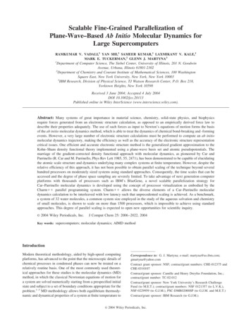
Plane-Wave–Based Ab Initio Molecular Dynamics2011Figure 1. Schematic flowchart of the implementation of the CP algorithm.of which is required before a scalable parallel algorithm can bedeveloped. The basic objects are the n s , occupied, real valuedelectronic states, { i (r)}, and their corresponding complex valuedplane-wave expansion coefficients, { i (g)}, which possess thesymmetry { *i (g)} { i ( g)}. Each state in real space, i (r),is represented by a 3D array (N N N) of real numbersassuming a cubic simulation cell for simplicity (L x L y L z ).Although the g-space representation should, in principle, be adense N N N array, a spherical cutoff is employed, 21 兩g兩 2 E cut, which confines the nonzero elements to lie within a sphere ofradius proportional to N/4. In general, the electron density in realspace, (r), is similarly represented by a single 3D array ofdimension N N N, with Fourier coefficients, (g). Like i (g), the nonzero elements of (g) are also contained within asphere but this time with radius proportional to N/ 2 (i.e., becausethe density is equal to i 兩 i (r)兩2). In general, the real spacerepresentations can be said to be “dense” while the reciprocalspace representations are comparatively sparse. Note, while employing sparse matrices reduces computation and communication,it also poses tricky load balance issues in parallel (i.e., someportions of reciprocal space have more nonzero data values thanothers).Having described the data dependencies, the states and theelectron density are shown, pictorially in Figure 2, evolving alongthe steps of the algorithm described in the previous section, whichis now divided into IX Phases. The algorithm begins with thereciprocal-space expansion coefficients of the states, { i (g)},which satisfy the orthogonality condition of eq. (16). In Phase I,Figure 2. A serial view of the CPAIMD algorithm, showing data dependences.

2012Vadali et al. Vol. 25, No. 16each state is transformed into its Cartesian or “real”-space” representation via 3D FFTs (Phase I), to yield the functions { i (r)} onthe real-space grid. The real-space representations of all states arethen squared and summed to obtain the electron density, (r) in the“Reduction” operations of Phase II. With (r) in hand, the Fouriercoefficients of the electron density, (g), can be obtained via aninverse 3D FFT.Two independent computations are now performed using theelectron density and its Fourier coefficients, respectively. First, theexchange-correlation energy, and its contribution to the KS potential are determined from the density in real space (Phase III).Second, the Hartree and local external energies are computed usingthe Fourier coefficients of the density (Phase IV) along with thecontribution of these two terms to KS potential, which is expressedon the same size reciprocal space as that describing the density, (g). The Hartree and local external contributions to the KSpotential are then transformed back into real space via 3D FFTs(Phase V) and added to the real space KS contribution determinedin Phase III.The two independent computational threads rejoin in Phase VI.In Phase VI, each state in real space (dense array of N N N)is multiplied by the KS potential (dense array of N N N) andFourier Transformed back into reciprocal space to generate theforce due to Hartree, local external, and exchange correlationenergies in reciprocal space. In

of the ab initio molecular dynamics method, which is able to treat the dynamics of chemical bond-breaking and -forming events. However, a very large number of electronic structure calculations must be performed to compute an ab initio molecular dynamics trajectory, making the efficiency as well as the accuracy of the electronic structure .