Transcription
Nuclear Medicine and Biology 30 (2003) 833– 844www.elsevier.com/locate/nucmedbioA review of graphical methods for tracer studies and strategies toreduce biasJean Logan*Chemistry Department, Brookhaven National Laboratory, Upton, NY 11973, USAAbstractGraphical techniques provide simple methods for the analysis of data from tracer studies. They provide considerable ease of computationcompared to the optimization of individual model parameters in the solution of the differential equations generally used to describe thebinding of tracers. The theoretical work of Patlak which was applied to irreversible tracers formed the basis for extensions of graphicaltechniques to reversibly binding tracers. The advantage of graphical methods is that they are not dependent upon a particular model structurebut provide a measure of tracer binding that can be interpreted in terms of a model structure if desired. They provide a visual way todistinguish the type of binding whether reversible or irreversible in the initial studies of new ligands. Conditions under which the graphicaltechniques can be applied are considered as well as problems encountered with slow binding components. One problem in the use of thesemethods particularly the method for reversible tracers is the bias generated due to the presence of statistical noise. Some recently proposedtechniques for reducing the noise are considered. 2003 Elsevier Inc. All rights reserved.1. IntroductionPET and SPET cameras record the time variation oflabeled tracer within the body after its introduction generally as a bolus injection. In order to convert this timesequence of radioactivities into one or more numbers thatare related to actual physiological processes, it is necessaryto apply compartmental models. These models are certainlyoversimplifications of the true physiology but neverthelessthey allow the estimation of model parameters for the comparison of subjects under different experimental conditionsand/or belonging to different groups. In particular, modelsallow the separation of processes of primary interest such asfree receptor concentration from other processes related totracer uptake. Frequently parameter estimation is done by aniterative nonlinear least squares method requiring a measured plasma input function in which radioactivity of thetracer is measured separately from the metabolites. Thedifferential equations of the compartment models can belinearized and the model parameters can be estimated usingstandard techniques for linear equations without the requirement of an iterative search (for example the work of Evansand Blomqvist [2,3]). Graphical analysis is a further simplification of general linear methods - it converts the model* Tel.: 1-631-344-4391; fax: 1-631-344-7902.E-mail address: jlogan@bnl.gov (J. Logan).0969-8051/03/ – see front matter 2003 Elsevier Inc. All rights s into one equation evaluated at the time pointscorresponding to the scanning times and provides fewerparameters, namely a slope and intercept. The graphicalmethods are independent of any particular model structure, although the slope can be interpreted in terms of acombination of model parameters for some model structure. Graphical methods also require an input functionalthough in some instances a reference region can be usedin place of plasma input if it is devoid of the specificbinding sites. Graphical analysis (GA) methods havebeen developed for reversibly [4 –7] and irreversiblybinding tracers [1,8,9]. In the case of irreversible tracerssome fraction of the radioactivity is trapped at the binding site for the duration of the experiment. Reversibletracers on the other hand demonstrate uptake and lossfrom all compartments over the time of the study. Themethod for irreversible tracers was developed first - thetheoretical foundation was provided by Patlak [1,9]. Theextension to reversible systems developed by Logan [4]was based on the original work of Patlak. Further refinements have been made by Ichise [7]. The main problemwith the use of graphical methods is the bias in theestimated parameters due to noise [10]. Recently somemethods for dealing with noise have been proposed[11,12]. We present here a review of the graphical methods, and recent developments in strategies to improveparameter estimation by reducing the bias.
834J. LoganNuclear Medicine and Biology 30 (2003) 833– 8442. Graphical analysis of reversible tracersIn general the compartmental equations can be writtenusing Patlak’s notation, [1,9]dC̃ K̃C̃ Q̃Cp共t兲dt(1)where C̃ is the vector of compartmental concentrations attime t, K̃ is a matrix of the transfer constants betweencompartments, Q̃ is a vector of plasma to tissue transferconstants which generally consists of one nonzero component designated as K1. Cp(t) is plasma concentration ofunmetabolized tracer (the input function). Using ROI共t兲 Vp Ci 共t兲Vp where ROI(t) (region ofiinterest) represents the sum of radioactivities from all compartments and includes the plasma volume fraction, Vp. U nin Patlak’s original notation is the tranpose of the vectorof 1’s that allows the summation of radioactivities. IntegratingEq. (1), multiplying by Ũ nK-1 and rearranging gives冕t冕ROI共t 兲dt 共–Ũ n K̃ 1Q̃ Vp0冕Cp共t 兲dt 冕C 1共t兲k3O¡O k4C 2共t兲both C 1 (nonspecifically bound tracer) and C 2 (specificallybound tracer) occupy the same physical volume, the DV isgiven by冉冊K1k31 k2k4(3)where k 3 Bmaxk on , Bmax is the receptor density and k onis the ligand receptor association constant. The DV for a 1tissue compartment is given by K1/ k 2 where k 2 is thetissue to plasma efflux constant. The ratio k 3/k 4 Bmax /Kd is also referred to as the binding potential [13]. The Kdfrom in vivo imaging studies implicitly includes a factoraccounting for the fact that only free ligand can bind to thereceptor. (It is assumed that there is a very rapid nonspecificcomponent so that k on is given by fk on, where f is the freefraction [13]. There may in addition be a slow nonspecificcomponent.) In the presence of multiple independent binding components, for example different classes of receptors,ROI共t兲constant,(4)aplotofvsCp共t 兲dt 0ROI共t兲is linear with a slope given by,Ũ nK̃ 1 Q̃, the total tissue distribution volume. Since thelast term in Eq. (4) is not constant due to the timedependence of C̃(t), the requirement is that it becomeseffectively constant after some time t* so that with furtherincreases in t* there is no further increase in the slope. Thetotal tissue distribution volume is a measure of the capacityof the tissue to bind the tracer. If the tissue and plasma arein equilibrium, the distribution volume is given by the ratioof the tissue concentration to the plasma concentrationDV C /Cp, where C 1i Ci 共t兲. Carson et al. [14]have developed methods for achieving a steady statecondition by controlling the infusion of tracer after abolus injection. However if the tracer is given as a bolusinjection only, the ratio C /Cp is not equivalent to the DVsince it is also a function of terms governing the loss oftracer from tissue [4,14]. When the tracer is given as abolusinjection,theDVisgivenby冕 (2 tissue components)Cp共t 兲dt 0tROI共t 兲dt ROI共t兲where Ũ n K̃ 1Q̃ is the total tissue distribution volume. It isreferred to as a volume for historical reason, although it isnot actually a volume since an increase in the DV can bedue to an increased number of binding sites within the samephysical volume. For the 2 tissue compartment modelshown below冕冕tŨ n K̃ 1C̃Ũ n C̃ VpC̃ nK̃ 1 C̃becomesŨ nC̃ VpWhen0(2) 共 Ũ n K̃ 1Q̃ Vp兲 tt Ũ n K̃ 1C̃Cp共t兲ROI共t 兲dt ROI共t兲0K1O¡O k2t0冘Ũ nC̃冉 冘 冊K1k11 iwhere i refers to the typek2K -1of binding component, k i is a first order rate constant including the number of available binding sites similar to thedefinition of k 3 and k -i is the ligand receptor dissociationconstant. Thus an increase in the total DV can be due to anincrease in the number of tracer binding sites within thesame space as seen by the tomograph.Dividing both sides of (Eq. 2) by ROI(t) givesthe DV becomes冕C 共t兲dt/0 Cp共t兲dt [15]. This not a particularly useful0representation since the radioactivities can only be measured at finite times.The linearity of Eq. (4) is achieved when ŨTn K̃ 1C̃/ŨTnC̃approaches a constant value. For the 2 tissue compartmentmodel冉冊Ũ n K̃ 1C̃k3C 2共t兲11 k2k4k 4共C 1共t兲 C 2共t兲Ũ n C̃whereC 2共t兲13共C 1共t兲 C 2共t兲兲1 k 4/k 3(5)
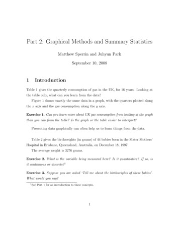
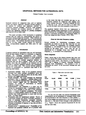
J. LoganNuclear Medicine and Biology 30 (2003) 833– 844Fig. 1. Typical uptake curves for 11C raclopride in the basal ganglia, aregion with D2 receptors, (upper curve) and cerebellum, a frequently usedreference region, lower curve. These are simulated data generated from ameasured plasma input function using model parameters K1 0.308mL/min/mL, k2 0.776 min-1, k3 0.3171 min-1 and k4 0.06 min-1, (DV 2.49 mL/mL) for the basal ganglia and K1 0.135mL/min/mL, k2 0.34 min-1, k3 0.10 min-1 and k4 0.24 min-1, (DV 0.562 mL/mL)for the cerebellum.835Patlak [1] pointed out that for t t a steady state conditionis reached for which C̃3K̃ 1 Q̃Cp(t). When this occurs,Ũ nK̃ 2 Q̃the intercept becomeswhich is constant. Ũ nK̃ 1 QC2 共t兲is changing slowly withHowever, when共C1 共t兲 C2 共t兲兲time and is close to its asymptotic value, a good estimateof the DV can be obtained for times before t , that is fort t* where t* t . An example is illustrated in Fig. 1for raclopride, a dopamine (DA) D2 antagonist that bindsto the D2 receptors in the basal ganglia. Raclopride is aligand that has been used extensively in PET research.Simulated data were generated using a measured plasmainput function with K1 0.308mL/min/mL, k2 0.776min-1, k3 0.3171 min-1 and k4 0.06 min-1, (DV 2.49mL/mL), for the basal ganglia and K1 0.135mL/min/mL, k2 0.34, k3 0.10 and k4 0.24 min-1, (DV 0.562 mL/mL) for the cerebellum, the reference region.These parameters were taken from a fit to experimentaldata. For both regions a two tissue compartment modelwas used. It is frequently necessary to use a two tissuemodel when fitting the reference region even thoughthere are no specific binding sites. The variation in t* forthese two regions is illustrated in Fig 2. For the basalganglia t* is on the order of 25 min and for the cerebellum t* is 15 min. In general t* depends upon k4 (and/ork2) which determines how fast the ratio C2/(C1 C2)reaches its asymptotic value (Eq. (5)). It also determinesthe required scanning length. The variation in the timedependence of the ratio C2/(C1 C2) as a function of k4 isFig. 2. Graphical analysis of the data from Fig 1. Time constant for start of the linear analysis for basal ganglia is 25 min and for cerebellum is 15 min. Theshorter time for the cerebellum is due to its more rapid kinetics as illustrated in Fig 1.
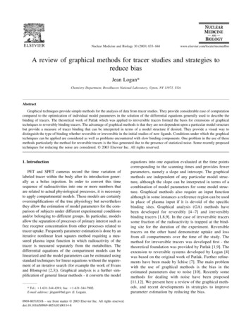
836J. LoganNuclear Medicine and Biology 30 (2003) 833– 844Fig. 3. Variation in the time dependence of the “intercept” of Eq. (4) with different values of k4, the receptor-ligand dissociation constant. Model parametersused in the simulations were K1 0.308mL/min/mL, k2 0.776 min-1, the k4 values used were 0.06, 0.04, 0.02, 0.005 min-1 (k3 was also varied to maintainthe same DV, 2.49 mL/mL). The asymptotic value for C2/(C1 C2) was 0.84.illustrated in Fig 3 for k4 values of 0.06, 0.04, 0.02, 0.005min-1 (keeping constant k3/k4 and the DV). The asymptotic value of C2/(C1 C2)is 0.84. For k4 0.06, and0.04 min-1, t* is on the order of 25 min. For k4 0.02min-1 the time required is longer 35 to 40 min. Todetermine t*, progressively longer initial times are useduntil the DV doesn’t change. Clearly with a very slow k4,for example k4 0.005 min-1 in Fig 3, the ratio C2/(C1 C2) has not reached the asymptotic value. When C2/(C1 C2) is less than the asymptotic value, the DV is underestimated, since the absolute value of the “intercept” is lessthan the true value. The graphical analysis for this example is illustrated in Fig 4 with k4 0.005. Taking anearly slope with t* 80 min and a final time of 120minthe DV is 2.01mL/mL an underestimate of 20%. Using allthe simulated data points from 80 to 255 min the DV isonly underestimated by 9%, (DV 2.26). With t* 220min a value close to the correct value is obtained,2.42mL/mL. The simulations were carried out to 255min. Two points emerge from this example. Even if t* isless than the time at which the effective steady state isreached, if a sufficient number of points are included inthe calculation after the this time, the error in the estimateof the DV is less. Secondly it will be difficult to obtaintrue estimates of the DV for ligands with slow kineticsthat are labeled with short half-life tracers such as C11.In this example if the total scanning time were only 1.5hours, the DV would be significantly underestimated.Fig. 4. Graphical analysis of simulated data in Fig 3 with K1 0.308mL/min/mL, k2 0.776, k3 0.0264 and k4 0.005 min-1, DV 2.49mL/mL. Using t* 80 min with end time 120 min the DV is underestimated by 20%. With t* 220min and end time 255 min, the DV is2.41mL/mL, close to the true value.
J. LoganNuclear Medicine and Biology 30 (2003) 833– 844When this occurs the DV can appear to be a function ofblood flow as in the example discussed below.In summary the operational equation for the GA ofreversible tracers using a plasma input is given by冕tROI共t 兲dt 0ROI共t兲 DV冕tCp共t 兲dt 0ROI共t兲 int(6a)where linearity is achieved for t* when the intercept (int) iseffectively constant. An alternative form of the GA equationis obtained from Eq. (4) by dividing by Cp(t) instead of theROI value giving冕tROI共t 兲dt 0Cp共t兲 DV冕tCp共t 兲dt 0Cp共t兲 int b(6b)in place of the plasma integral. This can be done by rearranging the graphical analysis equation for the referenceregion to solve for the plasma integral in terms of thereference region radioactivity. Rearranging Eq. (6a) whereREF is used in place of ROI gives冕tCp共t 兲dt 0Generally the DV ratio (DVR) or binding potential, whichcan be derived from the DVR are used for comparing datasets. The DVR is the ratio of the DV in a receptor region tothat of a reference region. This generally provides betterreproducibility on test/retest than comparing either the DVor the receptor parameter k3. If the DV of the referenceregion has one tissue compartment, then the binding potential (BP) can be derived from the DVR(7a)Substituting for the integral of the plasma in the equation forthe receptor ROI Eq. (6a) gives冕tROI共t 兲dt ROI共t兲䡠冕冤DVDV REFtREF共t 兲dt —int REFREF共t兲0ROI共t兲冥 int ROI .(7b)If the reference region is a one tissue compartmentmodel, then DVREF is given by K1 /k2 and intREF is –1/k2 .This, however, is not a requirement for the method. Forsimplicity of expression let intREF 1 1/k 2REF, whichin the case of a two tissue compartment model is given byEq. (5) so that1 REF k21k REF2冉1 k REF3k REF4冊 k REF共141. k REF/k REF兲43Replacing k 2REF with an average over subjects, k 2REF , then ROI共1 BP兲 REF冕ROI共t 兲dt 0 DVRROI共t兲冕冤twhere K1/k2 for ROI or REF, if this ratio is the same inboth tissues, which is a common assumption, thenBP DVR-1. However, in many cases the reference regionis not well described by a single tissue compartment so thatthe DVR contains in addition to the rapid nonspecific binding extra terms corresponding to a slower nonspecific binding component with equilibrium constant (NS),DVR 册REF共t 兲dt int REFREF共t兲 .0The problem with this formulation as discussed above isthat the true steady state condition must apply before linearity is achieved and this generally requires somewhatlonger times than when ROI is used in the denominator.DVR 冋冕1DV REFt03. Distribution volume ratio837tREF共t 兲dt REF共t兲/k tREF20 int ROI If and NS are the same in both tissues, DVR 1 fBP where f NS 1/(1 NS). The interpretation of the BPderived from the DVR is somewhat different in this casesince it is modified by the factor f NS.NS4. Graphical analysis using a reference regionWe can extend graphical analysis to obtain DV ratiosdirectly without blood sampling by using a reference region冉where the error term is DVRoperational equation is ROI共1 NS BP兲 . REF共1 NS REF兲ROI共t兲冕冥冊11 REF共t兲. The REFROI共t兲kREFk 22tROI共t 兲dt 0 DVRROI共t兲䡠冤冕tREF共t 兲dt REF共t兲/k REF20ROI共t兲冥 int (8)In many cases the term REF(t)/k 2 REF may be omitted. Fig 5
838J. LoganNuclear Medicine and Biology 30 (2003) 833– 844Fig. 5. The time variation of the “intercept” of the GA using a reference region for the raclopride example of Fig 3 with k4 0.06 and 0.02min-1. A somewhatlonger time is required for the slower dissociation (lower curve) to become constant.illustrates the time variation of the intercept for the racloprideexample given above with k4 0.06 and 0.02 min-1.An alternative form of this equation has been proposedby Ichise and Ballinger [6], a bilinear analysis where b andb correspond to intROI and –(DVR intREF) respectively inEq. (7b)冕tROI共t 兲dt 0ROI共t兲 DVR冕冤tREF共t 兲dt 0ROI共t兲冥 b REF共t兲ROI共t兲 b(8b)b and b become constant for t t*.5. Graphical analysis of irreversible tracersdTr Ũ n G̃C̃dtwhere G̃ is a matrix of transfer constants from the reversiblecompartments to the irreversible compartment and Tr is theconcentration in the trapped compartment. The operationalequation for the graphical analysis of irreversible tracers isROI共t兲 KiCp共t兲冕tCp共t 兲dt 0Cp共t兲 fVe Vpwhere Ki is the influx constant describing the transfer oftracer from the plasma compartment to the irreversible compartment. The term fVe corresponds to Ũ Tn (G̃K̃ 1 I)C̃/Cp(t). The “intercept” contains the fraction f of the tracer inthe reversible compartments that goes back into the plasmaand leaves the system [1]. Here ROI共t兲 Some tracers bind irreversibly, for example the monoamine oxidase (MAO) tracers [11C] L-deprenyl, and thedeuterium substituted [11C] L-deprenyl-D2 [16 –18] are suicide inhibitors for MAO B and similarly [11C] clorgylineand [11C]clorgyline-D2 irreversibly inhibit MAO A [19].Other tracers may appear irreversible over the course of thePET experiment because the ligand receptor dissociation isvery slow. In addition to Eq. (1) which describes the reversible parts of the system, the accumulation into the irreversible compartment is given by the general equation (1)(9)and Ve is given by冘C 共t兲 Tr.i冘C 共t兲/Cp共t兲 which for some time t t iiibecomes constant, that is, the steady state condition for thereversible components must apply. In the steady state condition f(t) also becomes constant. If the binding is notstrictly irreversible, that is if there is a slow loss from theirreversible compartment, then Eq. (9) can be modified totake this into account [9]. Using kb as a rate constant for theloss from the irreversible compartment and assumingkb Ki the graphical analysis becomes
J. LoganNuclear Medicine and Biology 30 (2003) 833– 844ROI共t兲 KiCp共t兲冕 0 fVe Vp .Cp共t兲In order to estimate the value of k b, the data should first beplotted according to Eq. (9). If it does not have a linearportion but appears concave, then k b 0. By increasing k bin small increments and plotting, a value can be found forwhich the graphical analysis is linear for some time t t .Patlak and Blasberg, [9] developed a graphical analysisfor irreversible systems using a reference region. This canalso be derived using Eq. (7a) for the plasma integral andsubstituting into Eq (9) and dividing by REF(t), 冕tREF共t 兲dt 0REF共t兲 int REFKiDV REFCp共t兲共 fVe Vp兲REF共t兲7. Problems with linear methods7.1. Using a plasma input functionThe differential equations used to describe movement oftracer between plasma and tissue compartments can belinearized so that the model parameters are more easilydetermined by solving a set of linear equations [2,3]. Forexample the differential equation for one tissue compartment modeldC 1共t兲 K 1Cp共t兲 k 2C 1dtThe slope is given by Ki/DVREF. Since Ve is defined as,冘 C 共t兲/Cp where the sum is over the reversible components in the region containing the trapped ligand, the last冘C 共t兲, neglecting Vp. When these termsterm becomes f1iK1 Ki. Obviously K1 must be greater than Ki. If k3 K1 –KiK1. then Ki is primarily dependent upon K1 and conveyslittle information about k3 (enzyme/receptor concentration). This is referred to as flow-limited and is a characteristic of the tracer not the method of analysis. e kb共t t兲Cp共t 兲dt KiROI共t兲 REF共t兲 共DV REF兲becomes冕iiiREF共t兲become constant, the graphical analysis equation applies.As with the reversible system this will be true for the steadystate case.6. Some problems with irreversible tracersA two tissue compartment model with one compartmentrepresenting the trapped component as illustrated belowCp共t兲K1O¡O k2C 1共t兲k3O¡C 2共t兲Ki k3K1 k3 . The ratio K1/k2 is notk2 k3K1 k3a function of blood flow [20], however, Ki depends uponblood flow since K1 is a function of blood flow andcapillary permeability [21]. An increase in Ki could bedue to either an increase in blood flow or an increase intracer binding. Since it is usually the change in tracerbinding that is of primary interest it is necessary toseparate these two processes. This means that Ki by itselfis not sufficient to characterize the ligand binding, K1needs to be determined also. If K1 is known, then k3has Ki 839C共t i兲 K 1ti0冕Cp共t兲dt k 2tiC 1共t兲dt i0where i are the error terms. Since the error terms are notstatistically independent, the parameter estimates may bebiased [22,23]. Feng [22] proposed a method for eliminatingthe bias but this applies to a particular model structure.Similarly the GA equation Eq. (6a) has been shown to givea biased estimates of the DV [10,11]. In traditional leastsquares estimation the independent variables are assumed tobe noise-free. Correlated noise appears in both the independent and dependent variables. Furthermore, as pointed outby Ichise [11] the GA method for reversible tracers Eq. (6a)contains the noisy tissue radioactivity as a denominator inthe independent variable, leading to a biased estimate. Logan [12] proposed a method for reducing the bias bysmoothing the data using the Feng 1 tissue compartmentmodel in two parts and then applying graphical analysis.This however is a more complicated calculation. Recentlytwo ideas have been proposed to reduce this bias whilemaintaining the simplicity of the calculation. One is the totalor perpendicular least squares (LS) that minimizes the perpendicular distance squared between the point and the fittedline [24]. This method takes into account the noise in theindependent as well as dependent variables. Ichise pointsout that the perpendicular LS method is the same as the totalLS method of Van Huffel and Vandewalle [25]. The methodproposed by Ichise [11] rearranges the GA equation into amultilinear regression form (Eq. (10) so that the independent variable is the integral of ROI which is subject to lessvariability than the ROI value,
840J. LoganNuclear Medicine and Biology 30 (2003) 833– 844Table 1Comparison of three formulations of the GA methodNoiseModelt CV% .09.26.14.120 1.3 1.74 7 104.3 20 23.12.28The coefficient of variation (CV) and %bias (estimated value - truevalue/true value 100) are given for three different formulations of thegraphical analysis method for reversible ligands.* Indicates that values 0 and 5 were eliminated for noise level .28(420/500).ROI共T兲 DVb冕t0Cp共t 兲dt 1b冕tROI共t 兲dt (10)0A third method was proposed by Ichise [11], but this isbased on a particular model and is not considered herealthough it seems to be more generally applicable. Usingthe previous raclopride example with DV 2.49, K1 0.308 mL/min/mL, k2 0.776, k3 0.317 and k4 0.06(min-1), the 3 linear methods, GA, GA with perpendiculardistance formulation (TLS) and the multilinear form ofEq. (10) (MLS) are compared in Table 1. Introducinggaussian noise (mean of zero and standard deviation ofone), that takes into account the scan duration ( ti) andisotope decay (B) with level of noise controlled by thescale factor Sc,Sc冉e tiROI共t i兲 t i冊1/ 2500 data sets were generated for each different value of Sc.Fig. 6 shows the results for the three methods in terms of theaverage and standard deviation. The results are given as aROIfunction of noise 具 f N典N,t i, whereROI共fN兲 N,ti 再 ROI共t兲 ROI 共t兲冎is the average of the absolute value of the differencebetween the noisy value and the true value, 兩 ROI共t兲兩divided by the true value, ROI T共t兲. Both forms of the GAunderestimate the DV with increasing noise, the TLSmethod is only slightly better than the GA method. TheMLS tends to a slight overestimate with noise but withincreasing variability. For the MLS method, estimatesoutside of reasonable values were excluded (values 0and 5). At low noise levels all methods are about thesame in terms of the coefficient of variation, CV, (SD/mean) and the bias (estimated value – true value). Atintermediate noise levels GA is 10% below the true valuewith 10% CV while the MLS gives an unbiased estimateof the mean but with a higher CV, 17%. At high noise theCV for MLS is 26% and the bias for GA is also on thatFig. 6. A comparison of the average value and standard deviation of the MLS, TLS and GA methods. The true value is indicated by the dashed line. TheGA method underestimates the DV with increasing noise. The TLS method is only slightly better. The MLS method has less bias with increasing noise butthe variability in terms of the standard deviation is increased over that of the GA and TLS.
J. LoganNuclear Medicine and Biology 30 (2003) 833– 844841Fig. 7. Results from the average of the GA and MLS methods. The standard deviation is less than with the MLS and the bias is less than the GA. The truevalue is indicated by the dashed line, the average is indicated by DV(MLS GA)/2.order, 23%. In order to improve the CV and reduce thebias in the GA method, an average of the DV for bothmethods was compared (Fig 7). This appears to extendthe noise range over which the bias and CV are reasonably small. For example the bias is 5% at noise level0.16 with CV 13% for the average of MLS and GA comparedto a bias of –15% and CV 11% for GA at the same noiselevel.Results for the GA method using the plasma tracerlevels in the denominator, Eq. (6b) are given in Table 2.The initial time t* was increased from 25 min as wasused for the original method Eq. (6a) to 35 min. ThisTable 2GA method for RAC example using Eq. Average DV, standard deviation (STD) and coefficient of variation (CV)for GA method of Eq. (6b) using plasma value instead of ROI in thedenominator.gave 5 points for the determination of the slope. The DVis slightly underestimated with 2.46 instead of 2.49for data without added noise. Using times from 30min the slope was 2.40 mL/mL. Interestingly there islittle variation in the average value over all noise levelsand the CV is comparable to the GA method Eq. (6a).The problem is that for many ligands it may not bepossible to find t* such that there are a sufficientnumber of points for which the intercept is changingslowly enough to allow a reasonable DV estimate.Raclopride happens to be a particularly good tracer inthis sense.These model independent methods are potentially useful forgenerating pixelwise images due to the speed of calculation aswell as the model independence. In order to reduce the bias andvariability, an average of values determined from some subsetof these different methods may be superior to any one of them.Also other methods that combine similar pixels to reduce noisemay be useful. Recently we used a method in the generation ofimages of the MAO tracer clorgyline combining pixels withina local region if they were within a certain fraction of the timeintegrated image (Logan et al, 2002). The idea is that pixelsthat are within close proximity and also within a certain rangeof the time integrated image are functionally related. Othertechniques for grouping pixels have been used to reduce noise[26].
842J. LoganNuclear Medicine and Biology 30 (2003) 833– 844Fig. 8. Simulations of 11C cocaine in the baboon cerebellum under conditions of high and low blood flow. The cerebellum has a slow nonspecific compartmentNSNSNSNSwith binding constants and min-1 with equilibrium binding constants k .025 and k k .04 min 1 with equilibrium binding constant NS k /NSk 0.625 and DV 共1 NS兲 3.57.8. Using a reference region inputAs with the plasma input function form of the GA equation, the reference region method is also susceptible tonoise. Using simulated ROI data without noise both reference region methods give very similar values for the DVR,4.44 and 4.41 for the bilinear and GA respectively (the“true” value is 4.43mL/mL). For comparison the Simplifiedreference tissue method (SRTM) [27] gives 4.68 for theDVR. The SRTM assumes that both receptor and referenceregion can be adequately described by a 1 tissue compartment model which is not true for this example. Data generated for the simulations above were used to illustrate thenoise properties of the DVR estimates. For low to moderatenoise both methods give similar results, however the bilinear method appears to be less susceptible to noise at thehigher levels DVR 4.10 0.21 and 3.88 0.42 for theGA and bilinear methods respectively. The DVR for theSRTM at this noise level was 5.02.9. Some problems with reversible tracers11C cocaine binds reversibly to the dopamine transporterand has been used in a number of studies [28 –30]. In recentbaboon studies we have encountered poor reproducibility ontest/retest which seems to be related to some extent to bloodflow. Studies done under different conditions of ventilationresulted in very large differences in bloo
ture. Graphical methods also require an input function although in some instances a reference region can be used in place of plasma input if it is devoid of the specific binding sites. Graphical analysis (GA) methods have been developed for reversibly [4-7] and irreversibly binding tracers [1,8,9]. In the case of irreversible tracers