Transcription
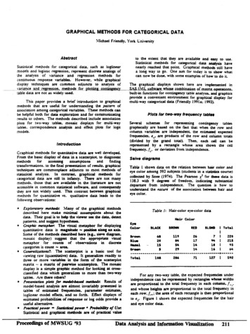
GRAPHICAL METHODS FOR CATEGORICAL DATA:1-fichael Friendly, York l:niversityAbstract --Statistical methods for categorical data. such as loglinearmodels and logistic regression, represent discrete analogs ofthe analysis of variance and regression methods for'ontinuous response variables. However. while graphicaldisplay techniques are common adjuncts to analysis ofvariance and regression. methods for plotting contingencytable data are not as widely used.This paper provides a brief introduction to graphicalmethods that are useful for understanding the pauem ofassociation among categorical variables. These methods canbe helpful both for data exploration and for communicatingresults to others. The methods described include associationplots for two-way tables, mosaic displays for multi-waytables. correspondence analysis and effect plots for logitmodels.IntroductionGraphical methods for quantitative data are well developed.From the basic display of data in a scatterplot. to transformations. to the final presentation of results, graphicaltechniques are commonplace adjuncts to most methods ofstatistical anal)·sis. In contrast, graphical methods forcategorical data are still in infancy. There are not manymethods. those that are available in the literature are notaccessible in common statistieal software. and consequendythey are not widely used. This contrast betWeen graphicalmethods for quantitative vs. qualitative data leads to thefollowing obser,·ations:Exploratory merluHJs: Many of the graphical methodsdescribed here make minimal assumptions about thedata. Their goal is to help the viewer see the data, deteetpauems. and suggest hypotheses. Graphic meraplulr. The visual metaphor for displayingquantitative data is magnitude - position alCJIII an axis.Some of the methods deseribed here (e.J., sieve diagram.mosaic display) suggest that the appropriate visualmetaphor for counts of observations in diseretecategories is count - area. Genera/it.alioru?: The scaUerplot is a basic: tool for,·iewing raw (quantitative) data. It generalizes readily tothree or more variables in the form of the seanerplotmatrix . a matrix of pairwise scaUerpJots. The mosaicdisplay is a simple graphic method for looking at eross·classified data which generalizes to more than two·waytables. Are there others? Presentalio11 pltlu f r mnluHlr. Results ofmodel-based analysis are almost invariably presented intables of estimated frequencies, parameter estimates,loglinear model effects, and so forth. Effect displays ofestimated probabilities of response or log odds provide auseful alternative. PracrU:al pDwer - SlllfUtillld power PrviJIIbility of Usr.Statistical and graphical methods are of pracacal valueto the extent that they are available and easy to use.Statistical methods for categorieal data analysis havenearly reaehed that point. Graphical methods still havea long way to go. One aim for today is to show whatcan now be done. with some examples of how to do iLThe graphical displays shown here are implemented inSASiiML software whose combinabon of matrix operationsbuilt-in funetions for contingency table analysi5. and graphiesprovide a convenient environment for graphical display formulti-way categorical data (Friendly 199la; 1992).Plots fOI' two-way frequency tabl Several sehemes for representing contingency tablesgraphically are based on the fact that when the row andcolumn variables are independent. the estimated expectedfrequencies, e,1 , are products of the row and column totals(divided by the grand total). Then. each cell can berepresented by a rectangle whose area shows the cellfrequency. f.1, or deviation from independence.Seive diagramsTab I shows data on the relation between hair color andeye color among 592 subjects (students in a statisties course)collected by Snee (1974). The Pearson x2 for these data is138.3 with 9 degrees of freedom; indicating substantialdeparture from independence. The question i5 how tounderstand the nacwe of the association betw- hair andeye color. Proceedings of MWSUG '93Table/: Hair-color eye-color dataHair ·ColorE: teColorBLACKIIIICMIRED.,68119201584SitZ6171414n 8Tot lFor any two-way table. the expected frequencies underindependence can be represented by rectangles whose widthsare proportional to the total frequency in each column. f 1 and whose heights are proportional to the total frequency ineach row,!,.; the arp of each rectangle is then proportionalto e,r Figure I shows the expected frequencies for the hairand eye color data.Data ADalysis and Information Visualization211
Hael.3 Blue8Association plot for 01.321.-447.2Z2D7.7two-way tablesIn the sieve diagram the foreground (rectangles) showsexpected frequencies; deviations from independence areshown by color and density of shading. The association plot(Cohen, 1980; Friendly, 199la) puts deviations fromindependence in the foreground: the area of each box ismade proportional to observed- expected frequency . For a two-way contingency table, the signedcontribution to Pearson -,;2 for cell i,j is d 11 (!;1 - e,) ' .J e,, so that x2 u,j - In .the IISSocitniott plot, each cell isshown by a rectangle that has (signed) height - dii andwidth - - The area of each rectangle is thereforeproportional to !,1 - e1r The rectangles for each row in thetable are positioned relative to a baseline representingindependence (d,1 0)' shown by a dotted line. Cells withobserved expected frequency rise above the line (and arecolored black); cells that contain less than the expectedfrequency fall below it (and are shaded red). Figure 3 showsthe association plot for the hair-eye color data. 1012118rr.nHair ColorBloelcFigure /:71Rea127Ilona512Expected frequencies under independence··R.ied\llo-yl and Schupbach (1983) propose a sieYfldiagram based on this principle. In this display the area ofeach rectangle is proportional to expected frequency andobserved frequency is shown by the number of squares ineach rectangle. Hence, the difference betwem observed andexpected frequency appears as the density of shading, usingcolor to indicate whether the deviation from independenc;e ispositive or negative. (In monochrome versions, positivedeviations are shown by solid lines, negative by brokenlines.) The sieve diagram for hair color and eye color isshown in Figure -····-···HAZEl.Sieve diagram: Hair Eye Color Dote-·-··BUCK81101111oREEHRED8LONOHair Color]Figure 3: Association plot for hair-eye dataSlue0.uFour-fold display for 2x 2 tables -SlackBrownHair ColorFigure 2: Sieve diagram for hair-eye dala212For a 2 x 2 table, the departUre from independence can bemeasured by the sample odds ,ario. 8 (/11 .' / 13}. if21; /22).The foru-fold display shows the frequencies in a 2 x 2 tablein a way that depicts the odds ratio. In this display thefrequency in each cell is shown by a quarter circle, whoseradius is proportional to .fi;1, so again area is proportionalto counL An association between the variables (odds ratio1) is shown by the tendency of diagonally opposite cellsin one direction to differ in size from those in the oppositedirection, and we use color and shading to show thisdirection. If the marginal proportions in the table differmarkedly, the table may first be standardized (using iterativeproportional fitting) to a table with equal margins but thesame odds ratio.Data Analysis and Information Vjsnalization'*Proceedings of MWSUG '93
Figure 4 shows aggregate data on applicants toschool at Berkeley for the six largest departmentsm 1973 classified by admission and gender. At issue iswhether the data show evidence of sex bias in admissionpractices (Bickel et al. 1975). The figure shows the cellfrequencies, but margins are equated in the display. Forthese data the sample odds ratio, Odds (AdmitJ:vlale) 1(Admit!Female) is 1.84 indicating that males are almost ·ice as likely in this sample to be admitted. The four·foldd1splay shows this imbalance clearly. We return to thesedata in the final section of lhis paper. raduate!i.Dli IDAdmit?: Yes E en::1 XenAdmit?: NoFigwe-t.X.J:F our·fold display for Berkeley admissionsMosaic displays for n-way tablesThe mosaic display. proposed by Hartigan & Kleiner (1981).represents the counts in a contingency table directly by tiles'-':hose area is proportional to the cell frequency. Thisd1splay generalizes readily to n-way tables and can be usedt.: display lhe residuals from various loglinear models.One form of this plot. called the t:DIUWued numricdisplay, is similar to a divided bar chart. The width of eacllcolumn of tiles in Figure 5 is proportional to the marginalfrequency of hair colors. Again, the area of eacll box isproportional to the cell frequency. and complete ndependence is shown when the tiles in each row all havethe same height.Detecting patternsIn Hartigan & Kleiner's (1981) original version (Figure S),all the tiles are unshaded and drawn in one color, so onlylhe relative sizes of the rectangles indicate deviations fromindependence. Friendly (1991 b) shows how to increase thevisual impact of the mosaic by using color and shading toreflect the size of the residual, and by reordering rows andc?lumns to make the pauem more coherent. The resultingd1splay shows both the observed frequencies and the pauernof deviations from a specified model.Proceedings of MWSUG '93IIII-0 0ooDDL--FigureS: Condensed column proportion mosaicDisplaying residuals. Figure 6 gives the extendedthe mosaic plot. showing the standardized deviation fromindependence, d,i by the color and shading of each rectangle:cells with positive deviations are drawn black, outlined withsolid lines, with shading slanted from upper left to lowerright (:--.: E to SW); negative deviations are drawn red,outlined with broken lines and shaded SE-:-.:W. Theabso!ute value of the deviation is portrayed by shadingdensaty: cells with absolute values less than 2 are empty;cells with ld1) 2: 2 are filled; those with ld,) 2: 4 are filled witha darker pauem. Standardized deviations are ofien referredto a standard Gaussian dislribution. t:nder the assumptionof independence, these values roughly correspond to two·tailed probabilities p .OS and p .000 I that a given valueof ld,) exceeds 2 or 4.Reordering categories. When the row or columnvariables are unordered, we are also free to rearrange thecorresponding categories in the plot to help show the natureof association. For example, in Figure 6, the eye colorcategories have been permuted so that the deviations fromindependence have an opposite-comer pattern, with positivevalues running from SW to :-IE comers, negative valuesalong the. opposite diagonal. Coupled with size and shadingof the tiles, the excess in the black-brown and blond·bluecells. together with the underrepresentation of brown-hairedblonds and people with black hair and blue eyes is nowquite apparent. Though the table was reordered based onthe d 1j values, both dimensions in Figure 6 are orderedfrom dark to light. suggesting an explanation for theassociation.Multi-way tablesThe condensed form of the mosaic plot generalizesreadily to lhe display of multi-dimensional contingencytables. Imagine that each ceil of the two-way table for hairand eye color is further classified by one or more additionalvariables-sex and level of education. for example. Theneach rectangle can be subdivided horizontally to show theData Analysis and lnfonnation Visualization213
----------------- ------,i- '------· ------, i.l! :Iby sex, fiUing the model IHairEye(SexJ allows us to see theextent to which the joint distribution of hair-color and eye·color is associated with su. For this model. the likelihood·ratio G2 is 29.3S on IS df(p .DIS), indicating some lack offit. The three-way mosaic. shown in Figure 7, highlights twocells: males are underrepresented among people with brownhair and brown eyes, and overrepresented among peoplewith brown hair and blue eyes. Females in these cells havethe opposite patterns, with residuals just shy of 2. The tl:,for these four cells account for 15.3 of the l for the model(HairEyel (Sex). Hence. except for these cells hair color andeye color appear unassociated with sex.IIIIIIIIIIIIIIIz---.IIII1----------------- I ---.1.!----------------,': ,, ----------------· ID ---'1IIIIIIIIIII·-I"'---·UHDFigure 6: Enhanced mosaic. reordered and shadedproportion of males and females in that cell. and each ofthose horizontal portions can be subdivided vertically toshow the proportions of people at each educational level inthe hair-eye-sex group.IFitting modelsWhen three or more variables are represented in the mosaic,we can fit several different models of independence anddisplay the residuals from that model. We treat thesemodels as null or baseline models. which may not fit thedata particularly well. The deviations of observedfrequencies from expected, displayed by shading, will oftensuggest terms to be added to to- an explanatory model thatachieves a beUer fit. The model of completeindependem:e:independence asserts that all joint probabilities areproducts of the one-way marginal probabilities:C 11mplere(I) for all i,j,k in a three-way table. This corTeSponds to theloglinear model (A)[BJ(CJ. Fitting this model puts allhigher terms. and hence all association among thevariables. into the residuals.Joint independelu:e: Another possibility is to fit the modelin which variable C is joinlly independent of variables Aand 8,(2)This corresponds to the loglinear model [ABl (CJ.Residuals from this model show the extent to whichvariable C is related to the combinations of variables Aand B but they do not show any association between Aand 8. ---,---,L--.2L.-JFigure 7: :\1osaic display for hair color, eye color, and sexSequential plots and models. The series of mosaicplots fiuing models of joint independence to the marginalsubtables can be viewed as partitioning the hypothesis ofcomplete independence in the full table.For a three-way table. the the hypothesis of completeindependence, H1,.868Cl can be expressed as(3)where H A Bl denotes the hypothesis that A and B areindependent in the marginal subtable formed by collapsingover variable C. and H(A.IJII!ICl denotes the hypothesis of jointindependence of C from the AB combinations. Whenexpected frequencies under each hypothesis are estimated bymaximum likelihood, the likelihood ratio G2s are additive:(4)For example, for the hair-eye data. the mosaic displays forthe (HairJIEyej marginal table and the (HairEyel (Sexj tablecan be viewed as representing the partitionFor example, with the data from Table l broken down214Data Analysis and Information VisualizationProceedings of MWSUG '93
df[lt.irl [bel[Hair, Eye] [Sex]915[Hair] [Eye] [S.xl146.4429.35179.79This partitioning scheme extends readily to higher·waytables.the OUT data set COORD requested in the PROCCORRESP step. The plot shows that both hair color andeye color vary from dark to light across Dimension 1.confuming the impression from the mosaic display.Dimension 2 reflects an independent association of red hairand green eyes. In faet, in the mosaic display we use scoreson the flfSt (largest) dimension to reorder the categories ofvariables in order to display the pattern of association mostclearly.o r------------------; -----------------;ICorrespondence analysisICorrespondence analysis is an exploratory technique relateda bat liAdsprincipal cor:ApoAer&ll analysistomultidimensional representation of the association betweenthe row and column categories of a two-way contingencytable. This technique fmds scores for the row and columncategories on a small number of dimensions that account forthe greatest proportion of the x for asaociation between therow and column categories. For graphical display, two orthree dimensions are typicaUy used to give a reduced rankapproximation to the data.------1IIIID : --- r-- - --- IIDIIIII ---- ------ ------ ---- 1.0O.SD.O -1.0Dlmen.,lFor a two-way table the scores for the row categories,namely .r,,. and column categories, y1,., on dimensionm I . .W are derived from a singular valuedecomposition of residuals from independence, expressed as. ofthe xl ·tn a the largest proporuon11. to account .ord,1 : v""small number of dimensions.Thus, correspondence analysis is designed to show howthe data deviate from expedition when the row and columnvariables are independent, as in the association plot andmosaic display. The association plot and mosaic displaydepict everv cell in the table, however. and for large tables itmay be d(fficult to see patterns. Correspondence analysisshows only row and column clllegories in the two (or three)dimensions which account for the greatest proportion ofdeviation from independence.In SAS Version 6. correspondence analysis isperformed using PROC CORRESP in SAS,"STAT. AnOLT data set from PROC CORRESP contains the rowand column coordinates, which can be plotted with PROCPLOT or PROC GPLOT. The program below reads thehair and eye color data into the data set COLORS, and callsthe CORRESP proeedure.data colors;in t BLACK BRONN RED 6Green7HazelA three- or higher-way table can be analyzed bycorrespondence analysis in several ways (Friendly, 1991a).One approach is called "stacking". A three-way table. ofsize I x J x K can be sliced into I two-way tables, eachJ x K. If the slices are concatenated vertically. the result isone two-way table. of size (/ x /) x K. In effect. the first twovariables are treated as a single composite variable, whichrepresents the main effects and interaction between theoriginal variables that were combined. Van der Heijden andde Leeuw ( 1985) discuss this use of correspondence analysisfor multi-way tables and show how each way of slicing andstacking a eontingency table corresponds to the analysis of aspecified log-linear model. In. particular. for the three-waytable that is reshaped as a table of size (I x /) x K. thecorrespondence analysis solution analyzes residuals from theloglinear model [ABJ [CJ.Etrect plots for logit modelslog mijk.proc correSP data colors out coord short;var BLACK BROWN RED BLOMDJid eye;The printed output from the CORRESP procedureindicates that over 98 'o of the x2 for association isaccounted for by two dimensions, with most of thatattributed to the flfSt dimension. A plot of the row andcolumn points, shown in Figure 8, can be constructed fromProceedings of MWSUG '93Multi-way tabhtsLoglinear and logit models generalize tests of association tothree- and. higher-way tables. A loglinear model expressesthe relationship among all variables as a model for the log ofthe expected cell frequency. for example, for a three-waytable, the hypothesis of no three-way association can beexpressed as the loglinear model, ;68Figure 8: Correspondenee analysis plotABCABAC-BC I' i A.i A.k A.ii A.i/c A.ikThe loglinear model treats the variables symmetrically: noneof the variables is distinguished as a response vanable.However, the association parameters may be difficult tointerpret, and the absence of a dependent variable makes itawkward to plot results iD terms of the loglinear model. Inthis case. correspondence analysis and the mosaic displayprovide a simpler way to display the panerns of associationin a contingency table.Data Analysis and Information Visualization215
On the other hand, if one variable can be regarded asa response variable then the effects of the other. independentvariables may be expressed as a logit model. For example,if variable C is a binary response, then the loglinear modelcan be expressed as an equivalent logit model,.Iog(miJl;mij7.) ( . C .c)( 1 .4C 1 .4C)"t-"2 "il -";2/31 U c.where a: 2.if.terms sum to zero.and /3: 2lf.c.( 1 BC BC)"it -A.j2because all lBoth loglinear and logit models can be lit using PROCCAT\100 in SAS. For logit models. plots of observed andpredicted togits provide an effective way to interpret a linedmodel. and are easily constrUcted from an output data setproduced by CAT:\-100. Fox (1987) describes generalmethods for constrUcting these plots for generalized linearmodels: see Friendly and Fox (1992) for further examplesand comparisons of these plots with mosaic displays.Example: Berkeley AdmissionsThe example below analyzes the Berkeley admissions databy deparunent to determine the source of the apparentgender bias in favor of males shown in the four-fold display(figure 4). The loglinear model [AdmitDeptl (AdmitGenderl[DeptGenderj allows for effects of both Gender andDeparunent on admission, and is equivalent to the logitmodellogit (Admit) a {J EPT {J ENDER(S)Vlodel (S) is lit using the statements below. TheRESPONSE statement is used to produce an output data set.PREOICT. for plotting.data t.rkeley do dept ·&· ·a , c·,-o , e , f ;do gender'Male ', 'F-1 '; do it 'AO.it',input freq aa;'Reject ;output;end; end; end;cards;51235312013&5322313207205279138351&9 19817202 391131 24429924 317""proc cataod order data data berke1 Ylweight freq resoonse I out predict nodel .O.it dept gender I 1 noit r The results of the PROC CAT:vJOD step show a strongeffect of Department. but none of Gender and a significantlack of lit.KAXI ·LIKELIHOODANALYSIS OF·YARIANCE TABLEDFChi 21670.0010LIKELIHOOD RATIO520.200.1011To interpret these results we plot the observed andpredicted values for each Dept-Gender group. The responsevariable has a simple, additive form (S) on the logit scale·Oog odds). but is easier to understand on the probabilityscale. One comprodlise is to plot results on the logit scale,adding a seconc1 scale showing probability values. The dataset PREDICT eontains observed LOBSJ and pr ictedLPREDJ values, and estimated standard erron LSEPREDJon both scales. The logit values have ,.TYPE 'FIJIICTION'.DEPT GENDER AIIIIIT TYPEAAAAAAtta1elta1 tta1eF-leF-1 F-1 assOA920.6210.379R jac l'lt08FUNCTION 1.5lt40.&24AO.it l'lt080.176R jec 1'11011FUNCTIONAO.U PliOIIPitED 0160.0990.0220.022To plot the lined logits. select the TYI'E 'FUNCTION'observations in a data step:data predict;set predict i f type 'fUNCTION' IA simple plot of predicted logits can then be obtained as aplot of pred c ept .r in a PROC GPLOT step.The plot displayed in Figure 9 uses the Annotate facility toadd 9 S'Yo onfidence limits, calculated as pred 1.96 sepred , and a probability scale at the right. Thesesteps are combined in a macro program. CATPLOT, used asfonows:7.catp1otCdata:predict. class gender, xc deltt.z 1.96, .,.,.sca1elThe effects shown in Figure 9 for each departmentcontradict the apparent gender bias shown in the aggregatedata; in fact. the predicted odds of admission is slighdyhigher for females than males. The resolution of thiscontradiction (an example of Simpson·s paradox) can befound in the large differences in admission rates amongdepartments.Men and women apply to diff departments differentially, and in these data women apply 1nlarger numbers to departments that have a low acceptancerate. The aggregate results are misleading because theyfalsely assume men and women are equally likely to apply ineach field. (This explanation ignores the possibility ofstrUctural bias against women. e.g., lack of resourcesallocated to deparunents that auract women applicants.)These effects may all be seen in Figure 1O. a mosaicdisplay of the data .showing observed frequencies andresidualsfrom the loglinearmodel(AdmitDept)216Data Analysis and Information VisualizationProceedings of MWSUG '93
Berlreley ACimi sion Oe ta08 ,. anG r.ttM 1.091 (tS" Cl)woe : loglt(AGmif) Oeon G.nGerAcknowledgements. I am grateful to John Fox andPaul Herzberg for careful readings of an initial draft of thispaper.z;Author's Address. For further information. contact !0 !-.sa · -1· . !-.51\fichael FriendlyPsychology Deparunent. Rm 210 BSBYork UniversityDownsview, 01'-o'T. Canada :\131 IP3Internet: FRIENDL Yil/ltl. Yol'kU. tA ·.75I '\--: CenCier References\.'\.· Ill r.,.,aie ICICIC1ac . 10".05 0Figure 9: Effects of Gender and Department on Admission[GenderDeptJ which asserts that admission and gender areconditionally independent, given department (equivalent tologit (Admit) "' pfEPT).The four large blockscorresponding to admission by gender show the greateroverall acceptance of males than females. Among admittedapplicants. however. there are larger proportions of womenin the departments (C-F) with low admission raleS. The lackof fit of model (AD) [GO[ is concentrated entirely inDepartment A. where a greater proportion of females isadmitted.I8orkole AGIII--. A.IID-.ot. -.o.,tJr : :J't -Jt:: jI. l-". J. lQi. -------------1IIIBleket, P. J ttamtnel. J. W. & O'Cunnell. J. W. (1915).Sex bias in graduate admissions: data from Berkeley.Science. 187, 398-403.Cohen. A. (1980). On the graphical display of the significantcomponents in a two-way contingency table. Commun.Scatisi.-Theor. Mech. A9. 1025-1041.Fox, J. (1987). Effect displays for generalized linear models.In C. C. Oogg (Ed.), Sociological Mechodology, /987,347-361. San Francisco: Jossey-Bass.Friendly, M. (1991a). SAS Sysrem for SuuiscU:al Graphics.Cary, NC: SAS Institute Inc.Friendly, M. (l991b), Mosaic displays for mulli·WGYconlingef!CJitab/u. York Univ.: Dept. of PsychologyReports. 1991. So. 19S.Friendly, M. (1992). SAS maero programs for statisticalgraphics. Psychome riko. in press.Friendly. M. and Fox. J. (1992). Interpreting higher orderinteraetions in Iog·Unear analysis: A picture is worth1000 numbers. York. Univ.: lost. for Social ResearchReport.Hartigan, J. A . and Kleiner. B. (1981 ). :\1osaics forcontingency tables. In W. F. Eddy (Ed.), ComputerScience and Slatislics: Proceedings of the I 3thSymposUurl on the [lllerface. Sew York: SpringerVerlag.Heijden. P. G. M. van der, and de leeuw. J. (198S).Correspondence analysis used complementary tologlinear analysis. Psychomerrika. 50, 429-447.Riedwyl. H . & Schupbach. :vt. (1983). Siebdiagramme:Grapbiscbe OarsteUung von Kontingenztafeln.Technical Report No. 12. Institute for MathematicalStatistics, University of Bern, Bern. Switzerland.Snee. R. D. (1974). Graphical display of two·waycontingency tables. The American ScaciscU:iDII. 28.9-12 .jIItJllaleFigure 10::VIosaic display of Berkeley admissions dataProceedings of MWSUG '93Data Analysis and Information Visualization217
Graphical methods for quantitative data are well developed. From the basic display of data in a scatterplot. to diagnostic methods for assessing assumptions and finding . Statistical methods for categorieal data analysis have nearly reaehed that point. Graphical methods still have a long way to go. One aim for today is to show what