Transcription
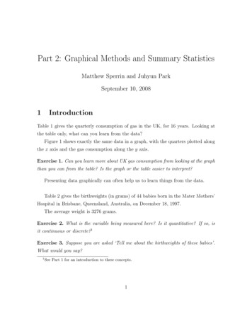
Graphical Methods for Uncertainty andSensitivity AnalysisRoger M. CookeDelft University of Technology, The NetherlandsJan M. van NoortwijkHKV Consultants, Lelystad, The NetherlandsContentsIntroduction1. A simple problem2.Tornado graphs3. Radar graphs4. Generalized reachable sets5. Matrix and overlay scatter plots6. Cobweb plots7. Cobweb plots for local sensitivity: Dikering reliability8. Radar plots for importance: Internal dosimetry9. Scatter plots for steering directional sampling: Uplifting and PipingConclusionsIntroductionGraphical methods play an important role in SA, since they provide a means of visualizing therelationships between the output and input factors. However, in complex problems, with many inputvariables, the problem of constructing useful graphical presentations becomes challenging, and thetypes of solutions become more varied. This chapter presents a number of familiar and perhaps not sofamiliar graphical tools which are used in SA. In chapter 2, Sampling methods, much use is made ofthe scatter plot for investigating pair-wise relationships and linearity, and here we present somemodifications of such plots, which allow more than two variables to be studied. We are all familiarwith the interpretation of the scatter plot, but in SA we are also interested on conditioning on thevalues of over input factors and on understanding the multi-dimensional relationships (very difficult tovisualize, and only possible through considering different projections).A literature search reveals very little in the way of theoretical development for graphical methods insensitivity and uncertainty analysis. Perhaps it is the nature of these methods that one simply ‘sees’what is going on. Apart from certain reference books, for example [Cleveland, 1993], the mainsources for graphical methods are software packages. Cleveland studies visualizing univariate,bivariate, and general multivariate data. Our focus however is not visualizing data as such, but rathervisualization to support uncertainty and sensitivity analysis.In this contribution we first choose a simple problem for illustrating generic graphical techniques. Thevirtue of a simple problem is that we can easily understand what is going on, and therefore we canappreciate what the various techniques are and are not revealing. Generic techniques are those thatcan be used for arbitrary problems, although screen size can become a limiting factor. The generictechniques discussed here are tornado graphs, radar plots, generalized reachable sets, matrix andoverlay scatter plots, and cobweb pots. Simple scatter plots have been presented in chapter two(section 4.5.2), and will not be discussed separately here. Where appropriate the software producingthe plots and/or analysis will be indicated.Having grasped what graphical techniques can do, it is instructive to apply them to real problemswhere we do not immediately 'see' what is going on. A problem concerning dike ring reliability is usedto illustrate the use of cobweb plots in identifying local probabilistically important parameters. Aproblem from internal dosimetry illustrates the use of radar plots to scan a very large set of parametersfor important contributors. Finally, a study of uplifting and piping failure mechanisms is used toillustrate the use of scatter plots and coplots in steering a Monte Carlo sampling routine. Of course,1
these problems themselves can only be treated in a cursory fashion, and the interested reader is referredto original reports for details.Uncertainty analysis codes, with or without graphic facilities, were benchmarked in a recent workshopof the technical committee Uncertainty Modeling of the European Safety and Reliability Association.The report [Cooke 1997] contains descriptions and references to the codes, as well as simple testproblems.1. A simple problemThe following problem1 serves to illustrate the generic techniques.Suppose we are interested in how long a car will start after the headlights have stopped working. Webuild a simple reliability model of the car consisting of three components: the battery (bat) the headlight lampbulb (bulb) the starter motor (strtr)The headlight fails when either the battery or the bulb fail. The car’s ignition fails when either thebattery or the starter motor fail. Thus considering bat, bulb and strtr as life variables:headlite min(bat, bulb)ignitn min(bat, strtr).The variable of interest is thenign-head ignitn - headlite.Note that this quantity may be either positive or negative, and that it equals zero whenever the batteryfails before the bulb and before the starter motor.We shall assume that bat, bulb and strtr are independent exponential variables with unit expectedlifetime. The question is, which variable is most important to the quantity of interest ign-head?2. Tornado GraphsTornado graphs are simply bar graphs arranged vertically in order of descending absolute value. Thespreadsheet add-on Crystal Ball performs uncertainty analysis and gives graphic output for sensitivityanalysis in the form of tornado graphs (without using this designation). After selecting a ‘targetforecast variable’, in this case ign-head, Crystal Ball shows the rank correlations of other inputvariables and other forecast variables as in Figure 1.Sensitivity ChartTarget Forecast: ign- 500.51Measured by Rank CorrelationFigure 1 Tornado graph.1This has been developed for the Cambridge Course for Industry, Dependence Modeling and RiskManagement [Cambridge Course for Industry 1998].2
The values, in this case rank correlation coefficients, are arranged in decreasing order of absolutevalue. Hence the variable strtr with rank correlation 0.56 is first, and bulb with rank correlation -0.54is second, and so on. When influence on the target variable, ign-head, is interpreted as rank correlation,it is easy to pick out the most important variables from such graphs. Note that bat is shown as havingrank correlation 0 with the target variable ign-head. This would suggest that bat was completelyunimportant for ign-head. Obviously, any of the global sensitivity measures of chapter two could beused instead of rank correlation (see also Kleijnen and Helton 1999).3. Radar GraphsRadar graphs provide another way of showing the information in Figure 1. Figure 2 shows a radargraph made in EXCEL by entering the rank correlations from Figure 1.Rank Correlation with eadliteignitnFigure 2 Radar graph.Each variable corresponds to a ray in the graph. The variable with the highest rank correlation isplotted furthest from the midpoint, and the variable with the lowest rank correlation is plotted closestto the midpoint. The discussion of the internal dosimetry problem in section 8 shows that the real valueof radar plots lies in their ability to handle a large number of variables.4. Generalized Reachable SetsThe method of generalized reachable sets [Bushenkov et al. 1995] involves approximating andvisualizing multi-dimensional sets given implicitly by a mapping. Although most often employed inmulticriteria analysis, its visualization facility as implemented in the MS WINDOWS software packageVISAN can be readily applied to problems like ign-head. The method enables the visualization of twovariables’ influence on a target variable (ign-head) by shaded contours (on screen the shades arecolored). In the present case the functional relations are extracted by sampling (bat, bulb, strtr),computing ign-head, and clustering the results. The clustering introduces numerical inaccuracies.Figure 3 shows shading of the value of bulb, with i-h (ign-head) on the vertical axis, and bat on thehorizontal axis. The shading at the point (i-h 1.015, bat 1.973) represents the range of values ofbulb found in the sample. We see that i-h bat, which indeed is obvious from the definitions. Further,i-h is positive only if bulb bat (the values of bat for i-h 0 and 4.445 bulb 5 have overwrittenthese values for bulb 4.445). From the definitions, we see if bat 1.973 and i-h 1.015, then bulb3
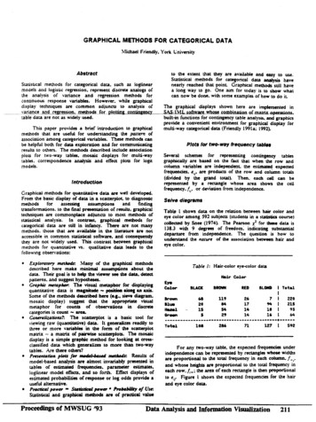
cannot be larger than 1.973 - 1.015 0.958. Figure 3 shows bat between 1.112 and 1.667. Figure 4shows the same information except that the roles of bulb and bat have been reversed. If we now takebulb 1.973, then we see i-h increases in bat if i-h 0 and decreases in bat if i-h 0 (this may bedifficult to see in black and white reproduction). In spite of numerical inaccuracies, these graphsprovide gradient type information; we can see what combinations of bat and bulb lead to increased ordecreased values of ign-head. The technique can deal with up to five variables by constructing twodimensional arrays of figures, but the interpretation of these figures is not easy.Figure 3 Relationships between bulb, bat, and ign-head.Figure 4 Alternative visualization of relationships between ign-head and bat and bulb.5. Matrix and overlay Scatter PlotsStatistical packages support varieties of scatter plots. For example, SPSS provides a matrix scatter plotfacility. Simulation data produced by UNICORN for 1000 samples has been read into SPSS to4
produce the plot matrix shown in Figure 5. We see pairwise scatter plots of the variables in ourproblem. The first row, for example, shows the scatter plots of ign-head and, respectively, bat, bulb,strtr, ignitn and headlite.IGN HEADBATBULBSTRTRIGNITNHEADLITEFigure 5 Matrix scatter plot.Figure 5 contains much more information than Figure 1. Let (a,b) denote the scatter plot in row a andcolumn b, thus (1,2) denotes the second plot in the first row with ign-head on the vertical axis and baton the horizontal axis. Note that (2,1) shows the same scatter plot, but with bat on the vertical and inghead on the horizontal axes.Although Figure 1 suggested that bat was unimportant for ign-head, Figure 5 shows that the value ofbat can say a great deal about ign-head. Thus, if bat assumes its lowest possible value, then the valuesof ign-head are severely constrained. This reflects the fact that if bat is smaller than bulb and strtr, thenignitn headlite, and ign-head 0. From (1,3) we see that large values of bulb tend to associate withsmall values if ign-head; if bulb is large, then the headlight may live longer than the ignition makingign-head negative. Similarly, (1,4) shows that large values of strtr are associated with large values ofign-head. These latter facts are reflected in the rank correlations of Figure 1.In spite of the above remarks, the relation between rank correlations depicted in Figure 1 and thescatter plots of Figure 5 is not direct. Thus, bat and bulb are statistically independent, but if we look at(2,3), we might infer that high values of bat tend to associate with low values of bulb. This however isan artifact of the simulation. There are very few very high values of bat, and as these are independentof bulb, the corresponding values of bulb are not extreme. If we had a scatter plot of the rank of batwith the rank of bulb, then the points would be uniformly distributed on the unit square.Figure 6 shows an overlay scatter plot.5
3002001000IGN HEAD-100STRTRIGN HEAD-200BULBIGN HEAD-300-100BAT0100200300400500600700Figure 6 Overlay of three scatter plots.Ign-head is depicted on the vertical axis, and the values for bat, bulb and strtr are shown as squares,triangles and diamonds respectively. Figure 6 is a superposition of plots (1,2), (1,3) and (1,4) ofFigure 5. However, Figure 6 is more than just a superposition. Inspecting Figure 6 closely, we see thatthere are always a square, triangle and diamond corresponding to each realized value on the verticalaxis. Thus at the very top there is a triangle at ign-head 238 and bulb slightly greater than zero.There is a square and diamond also corresponding to ign-head 238. These three points correspond tothe same sample. Indeed, ign-head attains its maximum value when strtr is very large and bulb is verysmall. If a value of ign-head is realized twice, then there will be two triples of squares-trianglediamonds on a horizontal line corresponding to this value, and it is impossible to resolve the twoseparate data points. For ign-head 0, there are about 300 realizations.The distribution underlying Figure 5 is six dimensional. Figure 5 does not show this distribution, butrather shows 30 two-dimensional projections from this distribution. Figure 6 shows more than acollection of two dimensional projections, as we can sometimes resolve the individual data points forbat bulb, strtr and ign-head, but it does not enables us to resolve all data points. The full distribution isshown in cobweb plots.6. Cobweb plotsThe uncertainty analysis program UNICORN contains a graphical feature that enables interactivevisualization of a moderately high dimensional distribution. Our sample problem contains six randomvariables. Suppose we represent the possible values of these variables as parallel vertical lines. Onesample from this distribution is a six-vector. We mark the six values on the six vertical lines andconnect the marks by a jagged line. If we repeat this 200 times we get Figure 7 below:6
Figure 7 Cobweb plot.The number of samples (200) is chosen for black-white reproduction. Onscreen, the linesmay be color coded according to the left-most variable: the bottom 25% of the axis is yellow, the next25% is green, then blue, then red. This allows the eye to resolve a greater number of samples andgreatly aids visual inspection. We can recognize the exponential distributions of bat, bulb and strtr.Ignitn and headlite, being the minimum of independent exponentials, are also exponential. Ign-headhas a more complicated distribution. The graphs at the top are the ‘cross densities’; they show thedensity of line crossings midway between the vertical axes. The role of these in depicting dependencebecomes clear when we transform the six variables to ranks or percentiles, as in Figure 8:7
Figure 8 Cobweb plot of ranks.A number of striking features emerge when we transform to the percentile cobweb plot. First of all,there is a curious hole in the distribution of ign-head. This is explained as follows. On one third of thesamples, bat is the minimum of {bat, bulb, strtr}. On these samples ignitn headlite and ign-head 0.Hence the distribution of ign-head has an atom at zero with weight 0.33. On one-third of the samplesstrtr is the minimum and on these samples ign-headlite is negative, and on the remaining third bulb isthe minimum and ign-head is positive. Hence, the atom at zero means that the percentiles 0.33 up to0.66 are all equal to zero. The first positive number is the 67-th percentile.Note the cross densities in Figure 8. One can show the following for two adjacent continuouslydistributed variables X and Y in a (unconditional) percentile cobweb plot2: If the rank correlation between X and Y 1 then the cross density is uniform If X and Y are independent (rank correlation 0) then the cross density is triangular If the rank correlation between X and Y -1, then the cross density is a spike in the middle.Intermediate values of the rank correlation yield intermediate pictures. The cross density of ignitn andheadlite is intermediate between uniform and triangular; and the rank correlation between thesevariables is 0.42.Cobweb plots support interactive conditionalization; that is, the user can define regions on the variousaxes and select only those samples which intersect the chosen region. Figure 9 shows the result ofconditionalizing on ign-head 0:2These statements are easily proved with a remark by Tim Bedford. Notice that the cross density is thedensity of X Y, where X and Y are uniformly distributed on the unit square. If X and Y have rankcorrelation 1, then X Y is uniform [0,2]; if they have rank correlation -1 then X Y 1; if X and Yare independent then the mass for X Y a is proportional to the length of the segment x y a.8
Figure 9 Conditioned cobweb plot of ranksNotice that if ign-head 0, then bat is almost always the minimum of {bat,bulb,strtr}, and ignitn isalmost always equal to headlite. This is reflected in the conditional rank correlation between ignitn andheadlite almost equal to 1. We see that the conditional correlation as in Figure 9 can be very differentfrom the unconditional correlation of Figure 8. From Figure 9 we also see that bat is almost alwaysless than bulb and strtr.Cobweb plots allow us to examine local sensitivity. Thus we can say, suppose ign-head is very large,what values should the other variables take? The answer is gotten simply by conditionalizing on highvalues if ign-head. Figure 10 shows conditionalization on high values of ign-head, Figure 11conditionalizes on low values (the number of unconditional samples has been increased to 1000).9
Figure 10 Conditional cobweb plot (high values for ign-head).Figure 11 Conditional cobweb plot (low values of ign-head).10
If ign-head is high, then bat, strtr and ignitn must be high. If ign-head is low then bat, bulb andheadlite must be high. Note that bat is high in one case and low in the other. Hence, we shouldconclude that bat is very important both for high values and for low values of ign-head. This is adifferent conclusion than we would have drawn if we considered only the rank correlations of Figures1 and 2.These facts can also be readily understood from the formulae themselves. Of course the methods comeinto their own in complex problems where we cannot see these relationships immediately from theformula. The graphical methods then draw our attention to patterns which we must then seek tounderstand. The following three sections illustrate graphical methods used in anger, that is, for real,difficult problems.7. Cobweb plots for local sensitivity: Dikering reliabilityIn this section we discuss a recent application in which graphical methods were used to identifyimportant parameters in complex uncertainty analyses. This application concerns the uncertainty indike ring reliability and was discussed in Cooke and van Noortwijk (1999). The dike ring in question isbuilt up of more than 30 dike sections. The reliability of each dike section i is modeled as:Reliabilityi Strengthi - Loadi.The reliability of the dikering is:relia Reliabilityring MIN{Reliabilityi}.The dike ring fails when relia 0. Figure 12 shows the unconditional percentile cobweb plot for reliaand 10 explanatory variables. From left to right the variables are: roughness (‘rough’);storm length (‘storm’);model factors for load, strength, significant wave period, significant wave height, and local waterlevel (‘mload’, ‘mstrn’, ‘mwvpr’, ‘mwvht’, and ‘mlwat’, respectively);wind (‘wind’);North Sea (‘nsea’);Rhine discharge (‘rhine’).For a further discussion of these variables and their role in determining reliability, we refer to Cookeand van Noortwijk (1999).11
Figure 12 Unconditional cobweb plot of reliability.Note from the cross densities tht nesa and rhine are negatively correlated, whereas nsea and wind arepositively correlated.Figures 13,14, and 15 show the results of conditionalizing, respectively, on the upper 5% of relia, the25 to 30-percentiles, and the bottom 5%. Failure occurs at the 2 percentile, hence Figure 15 showsconditionalization to ‘dangerous’ values of the dikering reliability. We make the followingobservations:12
Figure 13 Conditional cobweb plot (upper 5% of relia).Figure 14 Conditional cobweb plot (25-30% of relia)13
Figure 15 Conditional cobweb plot (lower 5% of relia). Very large values of relia are associated with very high values of mstrn and low values of storm;other variables are hardly affected by this conditionalization, and their conditional distributions arepractically equal to their unconditional distributions (i.e. uniformly distributed over percentiles). For values of relia around the 30-percentile, mstrn must be rather low, other variables are hardlyaffected by the conditionalization. For dangerous values of relia, nsea and wind must be high, other variables are unaffected by theconditionalization. For dangerous values of relia, the correlations wind-nsea and nsea-rhine are weaker than in theunconditional sample.We interpret “unaffected by the conditionalization” in this context as “unimportant for the values of‘relia’ on which we conditionalize. E.g. knowing that reliability is very high, we should expect thatstorm length is low and the model factor for strength is very high. With regard to other variables,knowing that relia is very high doesn’t affect our knowledge about what values these variables mighttake.This example shows that importance in the above sense is local. The variables which are important forhigh values of relia are not necessarily the same variables as those which are important for very lowvalues of relia.Intuitively, when we conditionalize an output variable on a given range of values, those input variableswhich are important for the given range are those whose conditional distributions differ most markedlyfrom their unconditional distributions. One convenient measure of this is the derivative of theconditional expectation of the input variable (Cooke and van Noortwijk, 1999). More precisely, theLocal Probabilistic Sensitivity Measure (LPSM) of variable X for variable Z when Z takes value z isthe rate of change of the expectation of X conditional on Z z. In the special case that Z is a linearcombination of independent normals, LPSM (X,z) is just the product moment correlation between Xand Z (i.e. it does not depend on z). If LPSM(X,z) 0, then the conditional expectation of X givenZ z is not changing in the neighborhood of z, which is taken to mean that X is probabilistically not14
important for Z z. Conversely large absolute values of LPSM(X,z) suggest that X is important forZ z. These notions are applied in the following example.8. Radar plots for Importance: Internal dosimetryAn ongoing joint study of the European Union and the US Nuclear Regulatory Commission aims toquantify the uncertainty for accident consequence models for nuclear power plants, based on structuredexpert judgment (Goossens, et al. 1997). The number of uncertain variables is in the order of 500. Notall of these can be considered in the Monte Carlo uncertainty analysis. Roughly 150 of the ‘mostimportant‘ variables must be selected for the Monte Carlo analysis. In this study there are a largenumber of output variables. In the example discussed here, there are 6 output variables correspondingto collective dose to six important organs. Moreover, we are not interested in all values of thesecollective doses, rather, we are interested in those variables which are important for high values ofcollective dose, for some organ. Hence, the LPSM(X, cdi) introduced above is applied to measure thesensitivity of input variable X for high values of collective dose to organ i, i 1, 6.There are 161uncertain variables which might in principle be important for high collective dose.With this number of input variables and output variables, and given current screen sizes, cobweb plotsare not useful. An EXCEL bar chart in Figure 16 shows LPSM(X, cdi), for the first 30 variables ( thefull set of variables requires a 7 page bar chart).15
Truncated bar chart, 30 input variables, 6 collective dosemeasurescd6Input -1.00E-010.00E 001.00E-012.00E-013.00E-01LPSM(X, cdi)Figure 16 Bar chart of the LSPM.This provides a good way of picking out the important variables. Bars extending beyond, say, -0.2 orbeyond 0.2 indicate that the corresponding variable is important for high values of a collective dose tosome organ. Of course the entire bar chart is too large for presentation here. Instead the radar chartsmay be used to put all the data on one page, as in Figure 17. Although compressed for the current pagesize, this figure enables us to compare all variables in one view. The same information in Bar chartform requires 7 pages. When printed on A3 paper the information in the 7 page b ar chart can be takenin at a glance.16
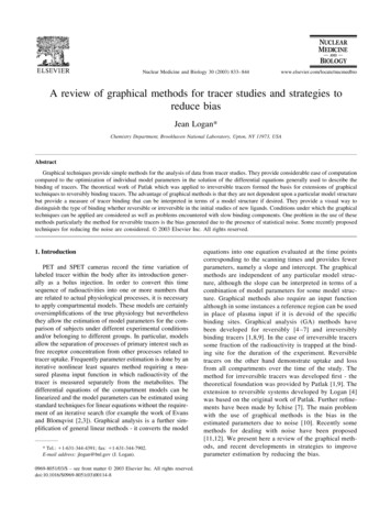
Sensitivity for High collective Dosecollective cd1dose cd2dose 5v260.00E v81 v80dose cd4dose cd5dose cd6Figure 17 Radar plot of LSPM.9. Scatter plots for steering for directional sampling: Uplifting and pipingAn important employment of graphical methods is for steering advanced Monte Carlo samplingroutines. One such routine is directional sampling. When applicable, it can significantly improve theestimation of low probabilities. This section describes the use of scatter plots for steering a directionalsampling routine. The data come from a study of dike failure due to uplifting and piping. For details,see Cooke and van Noortwijk (1999), and van Noortwijk et al. (1999).A dike fails owing to uplifting and piping when water tunnels under the dike erode the back face. Areliability function Z is defined for uplifting and piping such that failure occurs when Z 0. Failuredue to uplifting and piping is a low-probability event. It requires very high local water levels andmany other structural variables are important as well. Local water levels are determined by the Rhinedischarge and the North Sea water level. Z is a function of all these variables.Suppose we hold all other variables at their nominal values and consider the uncertainty in the Rhinedischarge Q and the North Sea level S. For given values of Q and S, we can determine whether or notpiping and uplifting occur. The probability of occurrence of uplifting and piping is thus determined bythe joint distribution of Q and S.In a full Monte Carlo exercise, we should have to sample very many times from the joint distributionof (Q,S) to build up a reliable estimate of the probability of uplifting and piping, since these are very17
rare events. In some cases we can transform (Q, S) to independent exponential variables. If we thenconsider these variables in polar coordinates (φ, r), then the following property holds: for a givensampled value φ , we can compute the probability of the set of r's for which uplifting and piping occur.The idea is then that we sample a direction φ and then compute the probability of uplifting and pipingin direction φ (see Ditlevsen and Madsen, 1996, Chapter 9). This gives us a relatively inexpensive wayof estimating the probability of uplifting and piping, when other variables are held at their nominalvalues. The question is how good is such an approximation?To answer this question graphical methods are brought into play. We first plot the failure hypersurfaceZ 0 in the transformed Q,S plane (Figure 18), where the failure region is the upper right part of thefigure. This is simply a scatter plot, conditional on nominal values of structural variables andconditional on Z 0. Thus, in Figure 18, only the "inherent" uncertainties in Q and S are taken intoaccount. If uncertainties in other variables were taken into account, this might cause failure to happenat other values (Q,S) than those shown in Figure 18. These new samples might render a failureprobability estimate based on Figure 18 unreliable.Limit state function z(x,y) 060Transformed maximum sea water level y50403020100010203040Transformed maximum discharge x5060Figure 18 The reliability function z(x,y) 0 in the (x,y)-plane for a dike section including 1000 samplesof (r (φ)sin(φ),r (φ)cos(φ)), where r (φ) is the zero of the reliability function, when only the inherentuncertainties in the river discharge and the sea water level are taken into account.To check this idea, we draw 10 000 from the uncertainty distributions of the structural variables, andfor each sample, we sample a direction and compute the probability of failure in the given direction asbefore. When we look at these in the transformed (Q, S) plane, we get the cloud of points in Figure 19.We may think of these points as projections onto the (Q, S) plane of points on the failure hypersurfacein the high dimensional space containing all uncertain variables. Alternatively, the cloud of pointsindicates how much the line in Figure 18 may vary as the other structural variables are sampled fromtheir uncertainty distributions.The dispersion of points in Figure 19 indicates that the failure probability is greatly influenced by theother structural variables. Reliable estimates of the failure probability using the two-dimensionaldirectional sampling method sketched above, still require about 1000 000 samples. For this reason, thedirectional sampling is extended to three dimensions, the third dimension being critical height U. U is afunction of several structural variables and reflects the water level which the dike can withstand.18
Limit state function z(x,y) 060Transformed maximum sea water level y50403020100010203040Transformed maximum discharge x5060Figure 19 The reliability function z(x,y) 0 in the (x,y)-plane for a dike section including 10 000samples of (r (φ)sin(φ),r (φ)cos(φ)), where r (φ) is the zero of the reliability function, when alluncertainties (including the inherent uncertainties of the critical height over the length of the dikesection) are taken into account.In order to calculate the probability of failure due to uplifting and piping, we transform (S, Q, U) tostandard independent exponential variabl
sensitivity and uncertainty analysis. Perhaps it is the nature of these methods that one simply 'sees' what is going on. Apart from certain reference books, for example [Cleveland, 1993], the main sources for graphical methods are software packages. Cleveland studies visualizing univariate, bivariate, and general multivariate data.