Transcription
Applied Mathematics, 2016, 7, 2336-2353http://www.scirp.org/journal/amISSN Online: 2152-7393ISSN Print: 2152-7385Hydraulic Reliability Assessment and OptimalRehabilitation/Upgrading Schedule forWater Distribution SystemsWei Peng, Rene V. MayorgaFaculty of Engineering, University of Regina, Regina, CanadaHow to cite this paper: Peng, W. and Mayorga, R.V. (2016) Hydraulic Reliability Assessment and Optimal Rehabilitation/Upgrading Schedule for Water Distribution Systems. Applied Mathematics, 7, Received: September 20, 2016Accepted: December 16, 2016Published: December 19, 2016Copyright 2016 by authors andScientific Research Publishing Inc.This work is licensed under the CreativeCommons Attribution InternationalLicense (CC BY en AccessAbstractThis paper develops an innovative approach to optimize a long-term rehabilitationand upgrading schedule (RUS) for a water distribution system with considering bothhydraulic failure and mechanical performance failure circumstances. The proposedapproach assesses hydraulic reliability dynamically and then optimizes the long-termRUS in sequence for a water distribution system. The uncertain hydraulic parametersare treated as random numbers in a stochastic hydraulic reliability assessment. Themethodologies used for optimization in a stochastic environment are: Monte CarloSimulation, EPANET Simulation, Genetic Algorithms, Shamir and Howard’s Exponential Model, Threshold Break Rate Model and Two-Stage Optimization Model.The proposed approach is conducted on a simulation model of water distributionnetwork in a computer by two universal codes, namely the hydraulic reliability codeand the optimal RUS code. The applicability of this approach is verified in an example of a benchmark water distribution network.KeywordsOptimization, Stochastic, Water Distribution, Rehabilitation, Upgrade, HydraulicReliability1. IntroductionWater distribution systems (WDSs) require huge investments in their construction andmaintenance. For this reason, it is an important need to improve their efficiency byways of minimizing their costs and maximizing the benefits. In the last several decades,a significant number of optimization methods have been developed using linear programming, dynamic programming, enumeration techniques, heuristic methods, andDOI: 10.4236/am.2016.718184 December 19, 2016
W. Peng, R. V. Mayorgaevolutionary techniques [1]. However, water distribution systems are so complex thatmost of the researches only address partial issues. For example, the previous optimalmaintenance schedule studies focused on either hydraulic capacity or mechanical performance failure by minimizing costs rather than the combination of them. The proposed study will develop such an innovative tool that considers the deterioration overtime of both structural integrity and hydraulic capacity of every pipe, and optimizes theRehabilitation & Upgrading Schedule (RUS) for an entire WDS.Hydraulic reliability assessment is used to study the deterioration over time of structural integrity and hydraulic capacity of WDSs; in other words, it is to study the mechanical failure and hydraulic failure over time. However, there are no universally accepted definitions for hydraulic reliability [2]. Here, we define hydraulic reliability as“the ability of a distribution system to meet the demands that are placed on it, wheredemands are specified in terms of: (i) the flow to be supplied, and (ii) the range ofpressure at which these flow rates must be provided [3].” Hydraulic failures occur whenthe demand nodes do not receive sufficient flow and/or adequate pressure, due to oldpipes with low roughness arising from corrosion and deposition, increases of demandand pressure head requirements, inadequate pipe sizes, insufficient pumping or/andstorage capabilities, etc. In addition, due to the fact that the demand is spatially andtemporally distributed, hydraulic failures at critical locations in the distribution systemmay be more important than the average system reliability [4]. Mechanical failures involve pipe breakage, pump failure, power outages, control valve failure, etc. Mechanicalfailure of the infrastructure components is also integrally linked with hydraulic failure.For instance, pipe breakage is a mechanical failure, and the occurrence of a pipe breakwill eventually result in insufficient flow rate and/or inadequate pressure head on thedemand nodes.In the previous researches, two methodologies were developed to compute the hydraulic reliability. One is the Monte-Carlo simulation (MCS) technique, which canbring more accurate reliability estimation [5] [6], but requires a large number of trialsto ensure accuracy thereby resulting in a computationally inefficient problem. Anotheris a linear probabilistic hydraulic model, called the first-order reliability method [7] [8],which can overcome the computationally inefficient problem in MCS, but has a loweraccuracy. Due to the rapid development of computer technology, the MCS has demonstrated its superiority in the hydraulic reliability computation. In this paper, the MCS ischosen to calculate the probabilistic problem of hydraulic reliability. A free simulationsoftware EPANET [9] is incorporated with this MCS to evaluate the nodal & system reliability of a water distribution system. It’s worth noting that the hydraulic reliabilityassessment here only refers to the hydraulic failure measurement but the mechanicalfailure measurement.The RUS optimization model is based on its hydraulic reliability assessment. It issubdivided into two stages. The first stage is the planning of upgrading and parallelingpipes due to hydraulic failure potential (such as demand and pressure); the secondstage is the schedule of repairing and replacing pipes due to mechanical failure poten2337
W. Peng, R. V. Mayorgatial (such as pipe breakage, pump, or aging of pipe). The first stage is domination dueto hydraulic failures that directly result in insufficient flow and/or inadequate pressure.On the other hand, mechanical failures only indirectly influence water supply on thedemand nodes. For example, the occurrence of one pipe break of a paralleling pipe system may only slightly lower the water flow rate and/or water pressure, but water supplymay still be sufficient.Previously, many research papers used various methodologies to study the optimalmaintenance schedule to the pipe networks focusing on either the hydraulic capacity orthe mechanical performance failure. Some of the earlier studies used linear programming [10] while the later studies utilized nonlinear programming [8] [11] to study thehydraulic failure for the optimal planning. Many of the recent literature applied geneticalgorithms for the determination of the lowest repairing or replacing costs [12] [13].Some researches had shown several advantages over more traditional optimization methods [14] [15] [16]. In the mechanical failure area, Shamir and Howard applied regression analysis to obtain a relationship for the breakage rate of a pipe as a function oftime [17]. Deb et al. suggested a failure probabilistic model to estimate miles of pipes tobe replaced on an annual basis [18]. Ascher and Feingold gave a threshold break ratefunction by using a statistical reliability model [19].This paper is to develop such innovative approach, with considers both hydraulicfailure and mechanical performance failure, to dynamically assess hydraulic reliabilityand then continue to find a best option for the long-term RUS of a water distributionsystem. This approach is conducted on a simulation model of water distribution network in a computer by two universal codes, namely the hydraulic reliability code andthe optimal RUS code, and it eventually will be applied in the real water distributionnetworks planning. The applicability of this approach is verified in an example of abenchmark water distribution network.2. Methodology2.1. Hydraulic Reliability AssessmentHydraulic failures occur when the demand nodes do not receive sufficient flow and/oradequate pressure, due to old pipes with low roughness arising from corrosion and deposition, increases of demand and pressure head requirements, inadequate pipe sizes,insufficient pumping or/and storage capabilities, etc. Mechanical failures involve pipebreakage, pump failure, power outages, control valve failure, etc. Mechanical failure ofthe infrastructure components is also integrally linked with hydraulic failure. For instance, pipe breakage is a mechanical failure, and the occurrence of a pipe break willeventually result in insufficient flow rate and/or inadequate pressure head on the demand nodes. Mathematically, the system hydraulic reliability equals 1 minus the systemfailure which shown in Figure 1. It notes that there has not a measurement method todirectly identify whether a failure is hydraulic or mechanical.2.1.1. Nodal Hydraulic Failure ProbabilityHydraulic failure at a given node occurs when the supplied flow or pressure is less than2338
W. Peng, R. V. MayorgaSystem Failure 1- System Hydraulic ReliabilityHydraulic FailureMechanical atePipe ComponentsFailurePipeBreakageOthersOthersFigure 1. Flowchart of system failure.the required minimum flow or the required minimum pressure at that node. Considering we will use EPANET for simulation that the hydraulic simulator always satisfieswater demand (because of applying the nodal mass balance equation) but not pressurehead, this approach automatically assumes that water demand is satisfied. The nodalmass balance equation can be expressed as:Di fij ( H i H j ) 0j Ω(1)i 1, 2, , N where Di is demand at node i; Hi is head at node i; Hj is head at node j; N is total number of the demand nodes with unknown heads; Ω is set of nodes connected directly tonode i; fij (*) is a nonlinear function relating the hydraulic loss and flow rate in thepipe connecting node i to node j. The nonlinear function used here is the HazenWilliams or the Colebrook-White equation.In the above equation, nodal pressure head is an unknown decision variable, andwater demands are state variables. This equation can be expressed in a more compactform:Fi ( H i 1, 2, , N0 i , Xi )(2)where Fi(*) is a vector of functions representing the mass balance at each node; Hi is avector of supplied pressure heads at each node; X i ( x1 , x2 , , xk )i is a vector of stateTvariables and k is the total number of variables. In the study of the hydraulic perfor-mance failure, we define water demands Di, pipe coefficients Ci, and tank/storage levelsLi as known state variables. Thus, the vector of state variables in this study can be ex-pressed as X i ( Di , Ci , Li ) ; T represents the matrix transpose operation. Moreover,T2339
W. Peng, R. V. Mayorgadue to uncertainty, those known state variables will be treated as random values. Eachrandom variable is expressed as a probability distribution, and then a random numbergenerator is used to generate the values of Di for each node, the values of Ci for eachpipe, and the values of Li for each tank/storage. Incorporation with EPANET, MonteCarlo simulation (MCS) technique can be applied to produce the random values ofpressure head.EPANET: EPANET is free public domain software developed by USEPA. It performsextended period simulation of hydraulic behavior within pressurized pipe networks [9].A network consists of pipes, nodes, pumps, valves and storage tanks or reservoirs.EPANET tracks the flow water in each pipe, the pressure at each node, the level of water in each tank during a simulation period. Running under Windows, EPANET provides an integrated environment for editing network input data, running hydraulic andwater quality simulations, and viewing the results in a variety of formats. In this study,water demands, pipe coefficients, tank/storage levels are inputting data during the simulation; pressure heads are outputs. We assume that pumps and valves are in goodoperation condition. The failure of pumps and valves is considered in the area of mechanical failure.Monte Carlo Simulation: Monte Carlo simulation involves repeated generation ofpseudovalues for the modeling inputs, drawn from known probability distributionswithin the ranges of possible values. In this study, this process will be completed bycomputer, where three random variables (water demand Di, pipe coefficients Ci, andtank/storage level Li) are produced synchronously at each time. The generated pseudovalues are then used as inputs for EPANET model to produce the supplied pressurehead values of Hi. The Monte Carlo simulation implementation in a node i includessteps: (1) development of the representative probability distribution functions for selected model input parameters; (2) generation of pseudovalues for each of the selectedinput parameters from the distribution developed in the previous step; (3) implementation of EPANET model with the pseudovalues to generate a pressure head value of Hi;(4) comparison of the calculated value of Hi with the minimum allowable head H iL ;(5) repeated application of the previous two steps; (6) presentation of the results, andanalysis of the results for decision making.In the above step (4) of the MCS procedure, we defined H iL as the minimum allowable head at a demand node. Thus, the probability of hydraulic performance failureat a demand node can be expressed as()H iLPi H P H i H iL DiS DiD 0 f ( H i ) dH i(3)where f ( H i ) is the probability density function of the supplied pressure head; DiS isthe supplied flow rate at the node i, and DiD is the water demand at the node i.2.1.2. Mechanical Failure ProbabilityMechanical failure involves pipe breakages and electric component failures (such aspump failure, power outages, control valve failure, etc). There are many factors thatmay cause pipe breaks, for instance, aging, physical bending stress, chemical and bio2340
W. Peng, R. V. Mayorgalogical corrosion, etc. Among these factors, aging, material type, dimension, and bedding quality are important factors in predicting pipe breakage. Here we demonstratetwo exponential break rate equations. Shamir and Howard’s exponential break ratemodel describes an exponential relationship between aging and breakage [17].A j ( t t0 )j P ( t ) j P j 1, 2, , M( t0 ) j epp(4)where Aj is the growth rate coefficient of the pipe j; P ( t ) j is the number of breaks per1000 ft. length of pipe j in year t; t is time in years; t0 is base year for the analysis (pipepinstallation year, or the first year for which data are available); M is total number ofpipes.In real situation, a primary cause of unreliability is the removal of water lines orpumps from service primarily due to breaks or power outages. A probability of an electromechanical component PkE (k 1, 2, , U; where U is total number of electriccomponents), such as a pump or a valve, being out of service can be included as another random variable that supported by historical data.2.1.3. System Hydraulic Reliability Assessment (See Figure 2)Different water demand has different importance. For example, a hospital water demand has the highest importance, and the water demand of a park area may have alower importance. We weight failure probabilities to reflect their different importanceFigure 2. Procedure of system hydraulic reliability assessment.2341
W. Peng, R. V. Mayorgaimpacts. Then, the system failure probability PS can be defined as the maximum individual failure probability in the system(PS MaxΧ Wi Pi H , W j PjP , Wk PkE , W F P F)(5)where Wi , W j , Wk , W F are weighting coefficients; Pi H is the probability of hydraulicperformance failure at the node i; PjP is the failure probability of pipe j; PkE is thefailure probability of electromechanical component k; P F is the fire flow failureprobability.The system hydraulic reliability RS is given byRS 1 PS .(6)2.2. Optimal Rehabilitation & Upgrading ScheduleThe long term planning of WDSs is an important issue for municipal agents. Theseagents pay special attention to improve the efficiency of their planning by the ways ofminimizing the costs and maximizing the benefits. However, water distribution systemsare so complex that most of the researches only address partial issues. For example, theprevious optimal maintenance schedule studies only focused on either hydraulic failureor mechanical failure by minimizing costs but the combination of them. This study willdevelop such an innovative model that considering the deterioration over time of bothstructural integrity and hydraulic capacity of every pipe, and optimizing the RUS for awhole WDS.The model identifies the network maintenance into the rehabilitation and the upgrading. It is subdivided into two stages (see Figure 3). The first stage is the planning ofFigure 3. Flowchart of two-stage method.2342
W. Peng, R. V. Mayorgaupgrading and paralleling pipes due to hydraulic failure potential (such as demand andpressure); the second stage is the schedule of repairing and replacing pipes due to mechanical failure potential (such as pipe breakage, pump, or aging of pipe). The firststage is domination due to hydraulic failures that directly result in insufficient flowand/or inadequate pressure. On the other hand, mechanical failures only indirectly influence water supply on the demand nodes. For example, the occurrence of one pipebreak of a paralleling pipe system may only slightly lower the water flow rate and/orwater pressure, but water supply may still be sufficient.It’s worth noting that we use “potential” to describe hydraulic failures and mechanical failures because we refer to those failures in future. Both prediction models of hydraulic failure and mechanical failure are based on the hydraulic reliability assessment.The hydraulic failure probability is assessed by the Monte Carlo Simulation, and thepipe breakage probability is computed by the Shamir and Howard’s exponential breakrate model (shown in Equation (4)). Because mechanical failure probability is obtainedin terms of historical data, the optimal upgrading results will not affect the pipe breakage probabilities except for the pipes that had been upgraded in the first stage.2.2.1. Rehabilitation Optimization ModelAlthough the pipe repair cost is much lower than the replacement fee, frequent breakswill result in the cumulative repair expense exceeding the replacement cost. Therefore,we need a methodology to find the critical (or threshold) break rate to determine thetiming of repair or replacement [19].If we assume that the pipe will be replaced at the time of the nth break (it also impliesthat for the previous (n 1) breaks only repairs have been performed), we can write thepresent worth of the total cost of the pipe as Tnn i 1Ci(1 β )ti Fn(1 β )tn(7)where β is the discount rate; ti is the time of the ith break measured from the installation year; Ci is the repair cost of the ith break; Fn is the replacement cost at timetn ; Tn is the present worth.For the total cost Tn at time tn to be a minimum, it must satisfy the conditionTn 1 Tn Tn 1 .(8)However, the critical check is to determine the first instance when the conditionTn 1 Tn holds true. Solving for( tn 1 tn ) , we have CF In n 1 n 1 FFn tn 1 tn n.In (1 β )(9)Recognizing tn 1 tn is the time between the nth and (n 1)th breaks or time interval for the occurrence of one break, we obtain the threshold break rate, Brkth, as the inverse of tn (where tn tn 1 tn ). The threshold break rate is defined as the breakrate between subsequent breaks.2343
W. Peng, R. V. MayorgaBrk th11 tn tn 1 tnIn (1 β ) CF In n 1 n 1 Fn Fn(10)Now, from the observed data for any given pipe we can derive a current break rate.Whenever the current break rate is equal to or more than Brkth, the pipe should be replaced. It is worth noting that the optimal rehabilitation schedule information will betransferred to the upgrading optimization process (shown in Figure 4).2.2.2. Upgrading Optimization ModelThe hydraulic reliability can indicate the hydraulic performance information for eachdemand node. If the hydraulic failure probability on a node is lower than the allowableprobability, the water provider should replace the inlet pipe with a larger diameter pipeor build a paralleling pipe. Then, the next few questions for the decision maker are: 1).Replace the existing pipeline by a bigger diameter pipeline or build a paralleling pipeline? 2) What size of pipe should be applied in this replacement or paralleling? 3) Theduration of the new inlet pipe that can transfer sufficient water?The design of water distribution systems is often viewed as a least-cost optimizationproblem in the previous literatures. The pipe diameters were considered as decision variables. Obviously other parameters should be considered as objectives in the optimization process, such as reliability, redundancy and water quality [20]. However, problemswith quantifying these objectives for use within optimization design models kept researchers concentrating on the single, least-cost objective. Therefore, the overall objective in the upgrading optimization in this paper is to minimize the total cost. The following formulation describes this objective:Figure 4. Example of distribution system.2344
W. Peng, R. V. MayorgaMinimize f C j ( R j , L j )m(11)jwhere C j ( R j , L j ) is the cost of pipe j with diameter Rj and length Lj; m is the numberof pipes that must be upgraded. The objective is subject to the following constraints:G ( H , D) 0(12)H L H HU(13)D D D(14)W L ( H , D) W ( H , D) W U ( H , D)(15)LUwhere Equation (12) refers to conservation of flow constraints and energy equations(loop equations); Equation (13) is head boundary constraints; Equation (14) is designedwater demand boundary constraints; Equation (15) represents general constraints including financial constraints.The decision on either replacement or paralleling pipeline is depended on cost, geographical situation, and the existing pipe condition. Some pipeline geographical conditions are not suitable for the laying of parallel pipelines that the only choice is to replacethe existing pipelines by larger diameter pipes. However, the geographical conditionconsideration of the pipe replacement planning is out of the scope of this study. In addition, we have to consider the duration of the upgraded pipeline. If one pipe neededupgrade because low hydraulic capability, simultaneously it was aging pipe that wouldbe replaced in the next few years, it was better to directly be replaced by a new largediameter pipe rather than to build a parallel pipeline.We assume the length of the term is l, the objective formulation is modified as follows Minimize fk 1 C jk ( R j , L j ) (1 β )ml j 1 k 1(16)where l is the length of the planning period; and k (k 1, 2, l) is the year index ofpipeline upgrading. The total cost includes the following components:C jk ( R j , L j )f 1 f 2(17)f 1 represents the pipeline costs including installation, paralleling, replacement andrepair costs; f 2 is the cost of setting up the construction plant and machinery.2.2.3. Optimization ProcedurePipe Roughness and Water Demand: The pipe roughness and the water demand aretwo model input parameters that vary over time. The pipe roughness increases overtime at a rate that varies according to the pipe type, water quality, and operation andmaintenance practices. To model the effect of aging on the carrying capacity of pipes,the equation of Sharp and Walsli [21] was used e a ( age ) C ( t ) 18.0 37.2 log o R (18)2345
W. Peng, R. V. Mayorgawhere C(t) is the Hazen-Williams coefficient in year t; eo is the roughness at the time ofinstallation (mm); a is the roughness growth rate (mm/year); and R is the pipe diameter(mm).The function developed by Dandy et al. [22] is used to predict nodal water demand.DGR Pt Di D0i 1 100 P0 tPREL(19)where D0j is the base year water demand for the node j and DGR is the annual percentage rate of increase in the base demand. DGR was assumed to follow demographic datapatterns closely, and so it was taken as the population growth rate with typical values ofabout 2 to 5; t is the time in years; Pt and P0 are the price per unit volume of water foryear t and the base year, respectively; PREL is the price elasticity of demand. A typicalrange of PREL values is 0.2 to 0.5. Generally it is advisable to increase the price ofwater in the last 1 or 2 years of the design period for the best results in order to delaythe need to upgrade the network. When there is adequate capacity after upgrading,prices can be reduced in order to utilize the system capacity as fully as possible and tomaximize economic efficiency. Other demand management options could be used, andself-evidently, the joint effect of all the demand management techniques deployedshould be considered.Genetic Algorithms: We have chosen the genetic algorithms (GA) as the optimization method. GA is a search technique used in computing to find exact or approximatesolutions to optimization and search problems. It is based on the mechanics of naturalselection and natural genetics that using biological techniques including inheritance,mutation, selection, and crossover [23]. GA provides a robust and efficient way tosearch complex parameter spaces for ever better solutions to an optimization problem[23]. Although there are no guarantees that a GA will actually attain the optimum, itgenerally finds one or more extremely good solutions with relatively little computational effort.The GA code can also be written by MATLAB. Moreover, EPANET simulation willbe run during the GA optimization process. The following steps give the details of theoptimization procedure for a repair schedule.Step 1. Use Equation (4) to calculate each pipeline’s break rate B(i, j); and use Equation (10) to compute each pipeline’s Brkth and then obtain the corresponding replacement year Yr(j), where i represents the time of year, and j is the pipe index.Step 2. Set i 0;Step 3. i i 1;Step 4. Run the hydraulic reliability model and calculate nodal hydraulic reliabilityR(i, j) for all studied nodes in a WDS in the ith year;Step 5. Compare the predicted hydraulic reliability with the minimum allowable hydraulic reliability Rm(i, j) at the ith year, to find the pipes to be upgraded P(i, j);Step 6. If the replacement year Yr(j) of the upgraded pipe is equal to or more than theplanning term N, then, no paralleling is considered;2346
W. Peng, R. V. MayorgaStep 7. Run Optimization Code (GA) to find optimal diameter pipe P(i, j, m) (wherem is the index of pipe diameter, both replacement and paralleling use this diameter index), with the objective of minimizing total cost, and subject to the constraint that theR(i, j) should be greater than the maximum of Rm(i, j) during the whole planning period N. The computation of R(i, j), of course, needs to run the hydraulic reliability prediction model;Step 8. If i N, then go to step 3;Step 9. Calculate the total cost and record the optimal rehabilitation and upgradingschedule.3. Example ApplicationFigure 4 shows a benchmark hypothetical water distribution system [24] that consistsof 16 pipes, 10 demand nodes, two tanks and one reservoir. Tables 1-4 demonstrate theinformation of system components.Due to we use the MCS to compute the nodal and system reliability, the iterativeprocess of random number generation of D, C, and L, and hydraulic simulation mustbe repeated a large number of times. According to the previous studies [6] [8], the optimal number of iterations is between 500 times to 3000 times. Because the results hadtiny different after 2000 iterations, we use 2000 iterations in this study.There are several probability distributions can achieve random number generation ofD, C, and L, such as normal, log-normal, uniform, Pearson and Weibull distributions.According to the literature, normal distribution is the most popular probability distribution that used in hydraulic studies [13] [14] [25] [26]. We also use normal distribution for random number generation of D, C, and L.The Shamir and Howard’s exponential break rate model (shown in Equation (4)) isused to compute the pipe breakage probability. The expected number of failures peryear per unit length of pipe Aj is uniformly assumed to be 0.122. The mean values ofTable 1. Node information.Node No.Elevation (ft)Mean demand (gpm)Min Allowable head N1042020502347
W. Peng, R. V. MayorgaTable 2. Pipe information.Pipe No.Length (ft)Diameter (in)Mean Hazen-Williams 22Table 3. Tank information.Tank 1Tank 2Base Elevation (ft)00Min Elevation (ft)525535Initial Elevation (ft)545550Max Elevation (ft)565570Tank Diameter (ft)35.749.3normal distribution of D, C, and L are obtained from Table 1 to Table 4. The coefficients of variation for D and L are assumed to be 0.2. According to the conclusion ofBao and Mays [6] that system reliability is somewhat insensitive to the type of probability distribution of pipe roughness when the coefficient of variation C is less than 0.4, weassume the coefficient of variation C is 0.4.The results of the nodal hydraulic performance failure probability, the pipe breakageprobability, and the system hydraulic reliability are shown in Table 5. From the results,we found i). The system reliability shows a great improvement
breakage, pump failure, power outages, control valve failure, etc. Mechanical failure of the infrastructure components is also integrally linked with hydraulic failure. For in-stance, pipe breakage is a mechanical failure, and the occurrence of a pipe break will eventually result in insufficient flow rate and/or inadequate pressure e- head on the d