Transcription
NOISeq: Di erential Expression in RNA-seqSonia Tarazona (starazona@cipf.es)Pedro Furió-Tarí (pfurio@cipf.es)María José Nueda (mj.nueda@ua.es)Alberto Ferrer (aferrer@eio.upv.es)Ana Conesa (aconesa@cipf.es)11 February 2016(Version 2.14.1)Contents1 Introduction22 Input data22.1Expression data . . . . . . . . . . . . . . . . . . . . . . . . . . . . . . . . . . . . . . . . . . . . . .2.2Factors . . . . . . . . . . . . . . . . . . . . . . . . . . . . . . . . . . . . . . . . . . . . . . . . . . .32.3Additional biological annotation. . . . . . . . . . . . . . . . . . . . . . . . . . . . . . . . . . . .32.4Converting data into a. . . . . . . . . . . . . . . . . . . . . . . . . . . . . . . . .4NOISeq object3 Quality control of count data253.1Generating data for exploratory plots. . . . . . . . . . . . . . . . . . . . . . . . . . . . . . . . .53.2Biotype detection . . . . . . . . . . . . . . . . . . . . . . . . . . . . . . . . . . . . . . . . . . . . .63.33.43.2.1Biodetection plot . . . . . . . . . . . . . . . . . . . . . . . . . . . . . . . . . . . . . . . . .63.2.2Count distribution per biotype7. . . . . . . . . . . . . . . . . . . . . . . . . . . . . . . . . . . . . . . . . . . . . . . . . . . . . . . . . . . .73.3.1Sequencing depth & Expression Quanti cationSaturation plot . . . . . . . . . . . . . . . . . . . . . . . . . . . . . . . . . . . . . . . . . .73.3.2Count distribution per sample. . . . . . . . . . . . . . . . . . . . . . . . . . . . . . . . .83.3.3Sensitivity plot . . . . . . . . . . . . . . . . . . . . . . . . . . . . . . . . . . . . . . . . . .9. . . . . . . . . . . . . . . . . . . . . . . . . . . . . . . . . . . . . . . .103.4.1Sequencing bias detectionLength bias . . . . . . . . . . . . . . . . . . . . . . . . . . . . . . . . . . . . . . . . . . . .103.4.2GC content bias3.4.3RNA composition. . . . . . . . . . . . . . . . . . . . . . . . . . . . . . . . . . . . . . . . .12. . . . . . . . . . . . . . . . . . . . . . . . . . . . . . . . . . . . . . . .123.5PCA exploration. . . . . . . . . . . . . . . . . . . . . . . . . . . . . . . . . . . . . . . . . . . . .133.6Quality Control report . . . . . . . . . . . . . . . . . . . . . . . . . . . . . . . . . . . . . . . . . .144 Normalization, Low-count ltering & Batch e ect correction144.1Normalization . . . . . . . . . . . . . . . . . . . . . . . . . . . . . . . . . . . . . . . . . . . . . . .4.2Low-count ltering . . . . . . . . . . . . . . . . . . . . . . . . . . . . . . . . . . . . . . . . . . . .164.3Batch e ect correction . . . . . . . . . . . . . . . . . . . . . . . . . . . . . . . . . . . . . . . . . .165 Di erential expression5.15.2NOISeq1518. . . . . . . . . . . . . . . . . . . . . . . . . . . . . . . . . . . . . . . . . . . . . . . . . .185.1.1NOISeq-real: using available replicates . . . . . . . . . . . . . . . . . . . . . . . . . . . . .195.1.2NOISeq-sim: no replicates available. . . . . . . . . . . . . . . . . . . . . . . . . . . . . .205.1.3NOISeqBIO . . . . . . . . . . . . . . . . . . . . . . . . . . . . . . . . . . . . . . . . . . . .20Results . . . . . . . . . . . . . . . . . . . . . . . . . . . . . . . . . . . . . . . . . . . . . . . . . . .215.2.1NOISeq output object . . . . . . . . . . . . . . . . . . . . . . . . . . . . . . . . . . . . . .215.2.2How to select the di erentially expressed features . . . . . . . . . . . . . . . . . . . . . . .225.2.3Plots on di erential expression results22. . . . . . . . . . . . . . . . . . . . . . . . . . . . .6 Setup251
1 IntroductionThis document will guide you through to the use of thecoming from next generation sequencing technologies.R Bioconductor package NOISeq, for analyzing count dataNOISeq package consists of three modules: (1) Qualitycontrol of count data; (2) Normalization and low-count ltering; and (3) Di erential expression analysis.First, we describe the input data format. Next, we illustrate the utilities to explore the quality of the countdata: saturation, biases, contamination, etc. and show the normalization, ltering and batch correction methodsincluded in the package. Finally, we explain how to compute di erential expression between two experimentalconditions.package.TheNOISeq and some of the plots included in the package wereNOISeq for biological replicates (NOISeqBIO) is also implemented in theThe di erential expression methoddisplayed in [1, 2].The new version ofNOISeqandNOISeqBIOmethods are data-adaptive and nonparametric.Therefore, no distributionalassumptions need to be done for the data and di erential expression analysis may be carried on for both rawcounts or previously normalized or transformed datasets.We will use the reduced Marioni's dataset [3] as an example throughout this document.experiment, human kidney and liver RNA-seq samples were sequenced.In Marioni'sThere are 5 technical replicates pertissue, and samples were sequenced in two di erent runs. We selected chromosomes I to IV from the originaldata and removed genes with 0 counts in all samples and with no length information available. Note that thisreduced dataset is only used to decrease the computing time while testing the examples. We strongly recommendto use the whole set of features (e.g. the whole genome) in real analysis.The example dataset can be obtained by typing: library(NOISeq) data(Marioni)2 Input dataNOISeq requires two pieces of information to work that must be provided to the readData function:the expressiondata (data) and the factors de ning the experimental groups to be studied or compared (factors). However,in order to perform the quality control of the data or normalize them, other additional annotations need to beprovided such as the feature length, the GC content, the biological classi cation of the features (e.g. Ensemblbiotypes), or the chromosome position of each feature.2.1 Expression dataThe expression data must be provided in a matrix or a data.frame R object, having as many rows as the numberof features to be studied and as many columns as the number of samples in the experiment.The followingexample shows part of the count data for Marioni's dataset: dney R1L2Liver R1L3Kidney R1L4Liver R1L6Liver R1L7Kidney 3111312101103040502121R2L2Kidney R2L3Liver R2L6Kidney113422547704282122015023949The expression data can be both read counts or normalized expression data such as RPKM values, and alsoany other normalized expression values.2
2.2 FactorsFactors are the variables indicating the experimental group for each sample. They must be given to thereadDatafunction in a data frame object. This data frame must have as many rows as samples (columns in data object)and as many columns or factors as di erent sample annotations the user wants to use. For instance, in Marioni'sdata, we have the factor Tissue , but we can also de ne another factors ( Run or TissueRun ). The levels of thefactor Tissue are Kidney and Liver . The factor Run has two levels: R1 and R2 . The factor TissueRun combines the sequencing run with the tissue and hence has four levels: Kidney 1 , Liver 1 , Kidney 2 and Liver 2 .Be careful here, the order of the elements of the factor must coincide with the order of the samples (columns)in the expression data le provided. myfactors data.frame(Tissue c("Kidney", "Liver", "Kidney", "Liver", "Liver", "Kidney", "Liver", "Kidney", "Liver", "Kidney"), TissueRun c("Kidney 1", "Liver 1", "Kidney 1", "Liver 1", "Liver 1", "Kidney 1", "Liver 1", "Kidney 2", "Liver 2", "Kidney 2"), Run c(rep("R1", 7), rep("R2", 3))) myfactors12345678910Tissue TissueRun RunKidney Kidney 1 R1LiverLiver 1 R1Kidney Kidney 1 R1LiverLiver 1 R1LiverLiver 1 R1Kidney Kidney 1 R1LiverLiver 1 R1Kidney Kidney 2 R2LiverLiver 2 R2Kidney Kidney 2 R22.3 Additional biological annotationSome of the exploratory plots inNOISeq package require additional biological information such as feature length,GC content, biological classi cation of features, or chromosome position. You need to provide at least part ofthis information if you want to either generate the corresponding plots or apply a normalization method thatcorrects by length.The following code show how the R objects containing such information should look like: head(mylength)ENSG00000177757 ENSG00000187634 ENSG00000188976 ENSG00000187961 6890 head(mygc)ENSG00000177757 ENSG00000187634 ENSG00000188976 ENSG00000187961 67.7 head(mybiotypes)ENSG00000177757 ENSG00000187634 ENSG00000188976 ENSG00000187961 ENSG00000187583"lincRNA" "protein coding" "protein coding" "protein coding" "protein coding"ENSG00000187642"protein coding" head(mychroms)3
0000187961ENSG00000187583ENSG00000187642Chr GeneStart GeneEnd1742614 7450771850393 8698241869459 8844941885830 8909581891740 9003391900447 907336Please note, that these objects might contain a di erent number of features and in di erent order than theexpression data. However, it is important to specify the names or IDs of the features in each case so the packagecan properly match all this information. The length, GC content or biological groups (e.g. biotypes), could bevectors, matrices or data.frames. If they are vectors, the names of the vector must be the feature names or IDs.If they are matrices or data.frame objects, the feature names or IDs must be in the row names of the object. Thesame applies for chromosome position, which is also a matrix or data.frame.Ensembl Biomart data base provides these annotations for a wide range of species: biotypes (the biologicalclassi cation of the features), GC content, or chromosome position. The latter can be used to estimate the lengthof the feature. However, it is more accurate computing the length from the GTF or GFF annotation le so theintrons are not considered.2.4 Converting data into a NOISeq objectOnce we have created in R the count data matrix, the data frame for the factors and the biological annotationobjects (if needed), we have to pack all this information into aNOISeq object by using the readData function.An example on how it works is shown below: mydata - readData(data mycounts, length mylength, gc mygc, biotype mybiotypes, chromosome mychroms, factors myfactors) mydataExpressionSet (storageMode: lockedEnvironment)assayData: 5088 features, 10 sampleselement names: exprsprotocolData: nonephenoDatasampleNames: R1L1Kidney R1L2Liver . R2L6Kidney (10 total)varLabels: Tissue TissueRun RunvarMetadata: labelDescriptionfeatureDatafeatureNames: ENSG00000177757 ENSG00000187634 . ENSG00000201145 (5088 total)fvarLabels: Length GC . GeneEnd (6 total)fvarMetadata: labelDescriptionexperimentData: use tion returns an object of Biobase's eSet class. To see which information is included in thisobject, type for instance: str(mydata)head(assayData(mydata) data)Note that the features to be used by all the methods in the package will be those in the data expressionobject. If any of this features has not been included in the additional biological annotation (when provided), thecorresponding value will be NA.It is possible to add information to an existing object. For instance,while using other packages such asTheaddDataDESeqnoiseq function accepts objects generatedpackage. In that case, annotations may not be included in the object.function allows the user to add annotation data to the object. For instance, if you generated thedata object like this: mydata - readData(data mycounts, chromosome mychroms, factors myfactors)4
And now you want to include the length and the biotypes, you have to use theaddDatafunction: mydata - addData(mydata, length mylength, biotype mybiotypes, gc mygc)IMPORTANT: Some packages such as ShortRead also use the readData function but with di erent input object and parameters. Therefore, some incompatibilities may occur that cause errors. To avoid this problem whenloading simultaneously packages with functions with the same name but di erent use, the following commandcan be used:NOISeq::readDatainstead of simplyreadData.3 Quality control of count dataData processing and sequencing experiment design in RNA-seq are not straightforward.From the biologicalsamples to the expression quanti cation, there are many steps in which errors may be produced, despite of themany procedures developed to reduce noise at each one of these steps and to control the quality of the generateddata. Therefore, once the expression levels (read counts) have been obtained, it is absolutely necessary to be ableto detect potential biases or contamination before proceeding with further analysis (e.g. di erential expression).The technology biases, such as the transcript length, GC content, PCR artifacts, uneven transcript read coverage,contamination by o -target transcripts or big di erences in transcript distributions, are factors that interfere inthe linear relationship between transcript abundance and the number of mapped reads at a gene locus (counts).In this section, we present a set of plots to explore the count data that may be helpful to detect these potentialbiases so an appropriate normalization procedure can be chosen. For instance, these plots will be useful for seeingwhich kind of features (e.g. genes) are being detected in our RNA-seq samples and with how many counts, whichtechnical biases are present, etc.As it will be seen at the end of this section, it is also possible to generate a report in a PDF le including allthese exploratory plots for the comparison of two samples or two experimental conditions.3.1 Generating data for exploratory plotsThere are several types of exploratory plots that can be obtained. They will be described in detail in the followingsections. To generate any of these plots, rst of all,object) to obtain the information to be plotted.computed for (argumenttype).datNOISeqfunction must be applied on the input data (The user must specify the type of plot the data are to beOnce the data for the plot have been generated withdatfunction, the plot willbe drawn with the explo.plot function. Therefore, for the quality control plots, we will always proceed like in thefollowing example: myexplodata - dat(mydata, type "biodetection")Biotypes detection is to be computed for:[1] "R1L1Kidney" "R1L2Liver" "R1L3Kidney" "R1L4Liver"[8] "R2L2Kidney" "R2L3Liver" "R2L6Kidney""R1L6Liver""R1L7Kidney" "R1L8Liver" explo.plot(myexplodata, plottype "persample")To save the data in a user-friendly format, thedat2savefunction can be used: mynicedata - dat2save(myexplodata)We have grouped the exploratory plots in three categories according to the di erent questions that may ariseduring the quality control of the expression data: Biotype detection:Which kind of features are being detected? Is there any abnormal contamination inthe data? Did I choose an appropriate protocol? Sequencing depth & Expression Quanti cation:to detect more features?Would it be better to increase the sequencing depthAre there too many features with low counts?Are the samples very di erentregarding the expression quanti cation? Sequencing bias detection:Should the expression values be corrected for the length or the GC contentbias? Should a normalization procedure be applied to account for the di erences among RNA compositionamong samples? Batch e ect exploration:Are the samples clustered in concordance with the experimental design orwith the batch in which they were processed?5
3.2 Biotype detectionWhen a biological classi cation of the features is provided (e.g. Ensembl biotypes), the following plots are usefulto see which kind of features are being detected. For instance, in RNA-seq, it is expected that most of the geneswill be protein-coding so detecting an enrichment in the sample of any other biotype could point to a potentialcontamination or at least provide information on the sample composition to take decision on the type of analysisto be performed.3.2.1 Biodetection plotThe example below shows how to use thedatandexplo.plotfunctions to generate the data to be plotted andto draw a biodetection plot per sample. mybiodetection - dat(mydata, k 0, type "biodetection", factor NULL)Biotypes detection is to be computed for:[1] "R1L1Kidney" "R1L2Liver" "R1L3Kidney" "R1L4Liver"[8] "R2L2Kidney" "R2L3Liver" "R2L6Kidney""R1L6Liver""R1L7Kidney" "R1L8Liver" par(mfrow c(1, 2)) explo.plot(mybiodetection, samples c(1, 2), plottype "persample")Fig. 1 shows the biodetection" plot per sample. The gray bar corresponds to the percentage of each biotypein the genome (i.e. in the whole set of features provided), the stripped color bar is the proportion detected in oursample (with number of counts higher thank),and the solid color bar is the percentage of each biotype withinthe sample. The vertical green line separates the most abundant biotypes (in the left-hand side, correspondingto the left axis scale) from the rest (in the right-hand side, corresponding to the right axis scale).Whenfactor NULL,the data for the plot are computed separately for each sample. Iffactoris a stringindicating the name of one of the columns in the factor object, the samples are aggregated within each of theseexperimental conditions and the data for the plot are computed per condition.In this example, samples incolumns 1 and 2 from expression data are plotted and the features (genes) are considered to be detected if havingk 0.R1L2Liver200.42000.40IG C genenon codingIG V genepolymorphic pseudogeneantisenseIG J geneprocessed transcriptrRNAlincRNAsnoRNAsnRNAmisc RNApseudogeneIG C genenon codingIG V genepolymorphic pseudogeneantisenseIG J geneprocessed transcriptrRNAmiRNAlincRNAsnoRNAsnRNAmisc RNApseudogeneprotein coding40protein coding%features01.3400.91.3%features6060% in genomedetected% in sample0.91.7800% in genomedetected% in sample801.7R1L1KidneymiRNAa number of counts higher thanFigure 1: Biodetection plot (per sample)When two samples or conditions are to be compared, it can be more practical to represent both o them inthe same plot. Then, two di erent plots can be generated: one representing the percentage of each biotype inthe genome being detected in the sample, and other representing the relative abundance of each biotype withinthe sample. The following code can be used to obtain such plots: par(mfrow c(1, 2)) explo.plot(mybiodetection, samples c(1, 2), toplot "protein coding", plottype "comparison")6
[1] "Percentage of protein coding biotype in each sample:"R1L1Kidney R1L2Liver91.091.7[1] "Confidence interval at 95% for the difference of percentages: R1L1Kidney - R1L2Liver"[1] -1.799 0.423[1] "The percentage of this biotype is NOT significantly different for these two samples (p-value 0.23Biotype detection over genome totalRelative biotype abundance in sample100R1L1KidneyR1L2Liver% in genome80Relative % biotypes604060402020Othersantisenseprocessed transcriptrRNAmiRNAlincRNAsnoRNAmisc RNAprotein codingIG C genenon codingIG V genepolymorphic pseudogeneantisenseIG J geneprocessed transcriptrRNAmiRNAlincRNAsnoRNAsnRNAmisc RNApseudogeneprotein codingsnRNA00pseudogene% detected features80Figure 2: Biodetection plot (comparison of two samples)In addition, the biotype comparison plot also performs a proportion test for the chosen biotype (argumenttoplot)to test if the relative abundance of that biotype is di erent in the two samples or conditions compared.3.2.2 Count distribution per biotypeThe countsbio" plot (Fig. 3) per biotype allows to see how the counts are distributed within each biologicalgroup. In the upper side of the plot, the number of detected features that will be represented in the boxplotsnorm FALSE) or the valuesnorm TRUE) The following code was used to draw the gure. Again, data are computedper sample because no factor was speci ed (factor NULL). To obtain this plot using the explo.plot function andthe countsbio" data, we have to indicate the boxplot" type in the plottype argument, choose only one of thesamples (samples 1, in this case), and all the biotypes (by setting toplot parameter to 1 or "global").is displayed. The values used for the boxplots are either the counts per million (ifprovided by the use (if mycountsbio dat(mydata, factor NULL, type "countsbio")[1] "Count distributions are to be computed for:"[1] "R1L1Kidney" "R1L2Liver" "R1L3Kidney" "R1L4Liver"[8] "R2L2Kidney" "R2L3Liver" "R2L6Kidney""R1L6Liver""R1L7Kidney" "R1L8Liver" explo.plot(mycountsbio, toplot 1, samples 1, plottype "boxplot")3.3 Sequencing depth & Expression Quanti cationThe plots in this section can be generated by only providing the expression data, since no other biologicalinformation is required. Their purpose is to assess if the sequencing depth of the samples is enough to detect thefeatures of interest and to get a good quanti cation of their expression.3.3.1 Saturation plotThe Saturation" plot shows the number of features in the genome detected with more thankcounts withthe sequencing depth of the sample, and with higher and lower simulated sequencing depths. This plot can be7
74113343074347233polymorphic pseudogene86misc RNA129miRNAnon coding45lincRNA3IG V gene175IG J geneantisense1IG C gene100010010snoRNAsnRNArRNApseudogeneprotein codinginfobioprocessed transcript0Expression valuesR1L1KidneyFigure 3: Count distribution per biotype in one of the samples (for genes with more than 0 counts). At the upperpart of the plot, the number of detected features within each biotype group is displayed.generated by considering either all the features or only the features included in a given biological group (biotype),dat and then weexplo.plot function.if this information is available. First, we have to generate the saturation data with the functioncan use the resulting object to obtain, for instance, the plots in Fig. 4 and 5 by applyingThe lines show how the number of detected features increases with depth. When the number of samples to plot is1 or 2, bars indicating the number of new features detected when increasing the sequencing depth in one millionof reads are also drawn. In that case, lines values are to be read in the left Y axis and bar values in the rightY axis. If more than 2 samples are to be plotted, it is di cult to visualize the newdetection bars , so only thelines are shown in the plot. mysaturation dat(mydata, k 0, ndepth 7, type "saturation") explo.plot(mysaturation, toplot 1, samples 1:2, yleftlim NULL, yrightlim NULL) explo.plot(mysaturation, toplot "protein coding", samples 1:4)The plot in Fig. 4 has been computed for all the features (without specifying a biotype) and for two of thesamples. Left Y axis shows the number of detected genes with more than 0 counts at each sequencing depth,represented by the lines. The solid point in each line corresponds to the real available sequencing depth. Theother sequencing depths are simulated from this total sequencing depth. The bars are associated to the right Yaxis and show the number of new features detected per million of new sequenced reads at each sequencing depth.The legend in the gray box also indicates the percentage of total features detected with more thank 0countsat the real sequencing depth.Up to twelve samples can be displayed in this plot. In Fig. 5, four samples are compared and we can see, forinstance, that in kidney samples the number of detected features is higher than in liver samples.3.3.2 Count distribution per sampleIt is also interesting to visualize the count distribution for all the samples, either for all the features or forthe features belonging to a certain biological group (biotype).Fig.6 shows this information for the biotype protein coding", which can be generated with the following code on the countsbio" object obtained in theprevious section by setting thesamplesparameter toNULL. explo.plot(mycountsbio, toplot "protein coding", samples NULL, plottype "boxplot")8
25001500New detections per million reads5000Number of detected features3400 3600 3800 4000 4200 4400GLOBAL (5088)0.10.20.30.40.50.60.70.8Sequencing depth (million reads) Left axis Right axis %detected0R1L1KidneyR1L2Liver85.480.9Figure 4: Global saturation plot to compare two samples of kidney and liver, respectively.Index3800360034003200Number of detected features4000PROTEIN CODING (4347)R1L1Kidney: 90.9% detectedR1L2Liver: 86.8% detected0.10.20.30.4R1L3Kidney: 91.1% detectedR1L4Liver: 86.5% detected0.50.60.70.8Sequencing depth (million reads)Figure 5: Saturation plot for protein-coding genes to compare 4 samples: 2 of kidney and 2 of liver.3.3.3 Sensitivity plotFeatures with low counts are, in general, less reliable and may introduce noise in the data that makes more di cultto extract the relevant information, for instance, the di erentially expressed features. We have implemented somemethods in theNOISeq package to lter out these low count features.The Sensitivity plot in Fig. 7 helps todecide the threshold to remove low-count features by indicating the proportion of such features that are presentin our data. In this plot, the bars show the percentage of features within each sample having more than 0 countsper million (CPM), or more than 1, 2, 5 and 10 CPM. The horizontal lines are the corresponding percentage offeatures with those CPM in at least one of the samples (or experimental conditions if thenotNULL).factorparameter isIn the upper side of the plot, the sequencing depth of each sample (in million reads) is given. Thefollowing code can be used for drawing this gure. explo.plot(mycountsbio, toplot 1, samples NULL, plottype "barplot")9
er010Expression values10000PROTEIN CODING (4347)Figure 6: Distribution of counts for protein coding genes in all samples.1000.40.50.40.5CPM 0CPM 10.50.40.5CPM 2CPM 50.50.50.5CPM idney0Figure 7: Number of features with low counts for each sample.3.4 Sequencing bias detectionPrior to perform further analyses such as di erential expression, it is essential to normalize data to make thesamples comparable and remove the e ect of technical biases from the expression estimation. The plots presentedin this section are very useful for detecting the possible biases in the data. In particular, the biases that can bestudied are: the feature length e ect, the GC content and the di erences in RNA composition. In addition, theseare diagnostic plots, which means that they are not only descriptive but an statistical test is also conducted tohelp the user to decide whether the bias is present and the data needs normalization.3.4.1 Length biasThe lengthbias" plot describes the relationship between the feature length and the expression values. Hence,the feature length must be included in the input object created using theplot is generated as follows.point of each bin is depicted in X axis.values (CPM ifreadDatafunction. The data for thisThe length is divided in intervals (bins) containing 200 features and the middleFor each bin, the 5% trimmed mean of the corresponding expressionnorm FALSE or values provided if norm TRUE) is computed and depicted in Y axis.If the numberof samples or conditions to appear in the plot is 2 or less and no biotype is speci ed (toplot global"), a10
diagnostic test is provided. A cubic spline regression model is tted to explain the relationship between lengthand expression. Both the model p-value and the coe cient of determination (R2) are shown in the plot as wellas the tted regression curve.If the model p-value is signi cant and R2 value is high (more than 70%), theexpression depends on the feature length and the curve shows the type of dependence.Fig. 8 shows an example of this plot. In this case, the lengthbias" data were generated for each condition(kidney and liver) using the argumentfactor. mylengthbias dat(mydata, factor "Tissue", type "lengthbias") explo.plot(mylengthbias, samples NULL, toplot "global")Liver10050Mean expression150100R2 52.28%p value: 0.0083p value: 0.00380R2 48.04%050Mean expression200150Kidney0e 003e 056e 050e 00Length bins3e 056e 05Length binsFigure 8: Gene length versus expression.More details about the tted spline regression models can be obtained by using thebelow: show(mylengthbias)[1] "Kidney"Call:lm(formula datos[, i] bx)Residuals:Min1Q Median3Q-85.40 -19.603.05 25.85Max74.83Coefficients: (1 not defined because of singularities)Estimate Std. Error t value Pr( t )(Intercept)121.348.62.490.0215 *bx1-35.052.2-0.670.5108bx2269.288.43.050.0064 **bx3-1301.1719.7 -1.81 0.0857 .bx46292.44655.41.350.1916bx5NANANANA--Signif. codes: 0 ***' 0.001 **' 0.01 *' 0.05 .' 0.1 ' 1Residual standard error: 48.6 on 20 degrees of freedomMultiple R-squared: 0.48,Adjusted R-squared: 0.37611showfunction as per
F-statistic: 4.62 on 4 and 20 DF, p-value: 0.00833[1] "Liver"Call:lm(formula datos[, i] bx)Residuals:Min1Q Median-51.8 -18.20.03Q21.3Max42.3Coefficients: (1 not defined because ofEstimate Std. Error t 154.04.12bx3-1141.7439.3 -2.60bx45758.12841.22.03bx5NANANA--Signif. codes: 0 ***' 0.001 **' 0.01singularities)Pr( t )0.170730.739520.00054 ***0.01716 *0.05624 .NA *' 0.05 .' 0.1 ' 1Residual standard error: 29.7 on 20 degrees of freedomMultiple R-squared: 0.523,Adjusted R-squared: 0.427F-statistic: 5.48 on 4 and 20 DF, p-value: 0.003823.4.2 GC content biasThe GCbias"
can properly match all this information. The length, GC content or biological groups (e.g. biotypes), could be vectors, matrices or data.frames. If they are vectors, the names of the vector must be the feature names or IDs. If they are matrices or data.frame objects, the feature names or IDs must be in the row names of the object. The

![Introduction to SEIR Models - Indico [Home]](/img/37/0.jpg)