Transcription
Introduction to differential formsDonu ArapuraMay 6, 2016The calculus of differential forms give an alternative to vector calculus whichis ultimately simpler and more flexible. Unfortunately it is rarely encounteredat the undergraduate level. However, the last few times I taught undergraduateadvanced calculus I decided I would do it this way. So I wrote up this briefsupplement which explains how to work with them, and what they are good for,but the approach is kept informal. In particular, multlinear algebra is kept toa minimum, and I don’t define manifolds or anything like that. By the time Igot to this topic, I had covered a certain amount of standard material, which isbriefly summarized at the end of these notes.My thanks to João Carvalho, John Crow, Matúš Goljer and Josh Hill forcatching some typos.Contents1 1-forms1.1 1-forms . . . . . . . . . . . . .1.2 Exactness in R2 . . . . . . . . .1.3 Parametric curves . . . . . . .1.4 Line integrals . . . . . . . . . .1.5 Work . . . . . . . . . . . . . . .1.6 Green’s theorem for a rectangle1.7 Exercise Set 1 . . . . . . . . . .223447892 2-forms2.1 Wedge product . . . . . . . . . . . . . . . .2.2 2-forms . . . . . . . . . . . . . . . . . . . .2.3 Exactness in R3 and conservation of energy2.4 Derivative of a 2-form and divergence . . .2.5 Poincaré’s lemma for 2-forms . . . . . . . .2.6 Exercise Set 2 . . . . . . . . . . . . . . . .10101113141516.3 Surface integrals183.1 Parameterized Surfaces . . . . . . . . . . . . . . . . . . . . . . . . 183.2 Surface Integrals . . . . . . . . . . . . . . . . . . . . . . . . . . . 201
3.33.43.54Surface Integrals (continued) . . . . . . . . . . . . . . . . . . . .Length and Area . . . . . . . . . . . . . . . . . . . . . . . . . . .Exercise Set 3 . . . . . . . . . . . . . . . . . . . . . . . . . . . . .Stokes’ Theorem4.1 Green and Stokes . . . .4.2 Proof of Stokes’ theorem4.3 Cauchy’s theorem* . . .4.4 Exercise Set 4 . . . . . .5 Gauss’ theorem5.1 Triple integrals . . .5.2 Gauss’ theorem . . .5.3 Proof for the cube .5.4 Gravitational Flux .5.5 Laplace’s equation* .5.6 Exercise Set 5 . . . .222427.2929303235.373737383941426 Beyond 3 dimensions*446.1 Beyond 3D . . . . . . . . . . . . . . . . . . . . . . . . . . . . . . 446.2 Maxwell’s equations in R4 . . . . . . . . . . . . . . . . . . . . . . 477 Further reading49A Review of multivariable calculus50A.1 Differential Calculus . . . . . . . . . . . . . . . . . . . . . . . . . 50A.2 Integral Calculus . . . . . . . . . . . . . . . . . . . . . . . . . . . 5211.11-forms1-formsA differential 1-form (or simply a differential or a 1-form) on an open subset ofR2 is an expression F (x, y)dx G(x, y)dy where F, G are R-valued functions onthe open set. A very important example of a differential is given as follows: Iff (x, y) is C 1 R-valued function on an open set U , then its total differential (orexterior derivative) is f fdx dydf x yIt is a differential on U .In a similar fashion, a differential 1-form on an open subset of R3 is anexpression F (x, y, z)dx G(x, y, z)dy H(x, y, z)dz where F, G, H are R-valuedfunctions on the open set. If f (x, y, z) is a C 1 function on this set, then its totaldifferential is f f fdx dy dzdf x y z2
At this stage, it is worth pointing out that a differential form is very similarto a vector field. In fact, we can set up a correspondence:F i Gj Hk F dx Gdy Hdzwhere i, j, k are the standard unit vectors along the x, y, z axes. Under this setup, the gradient f corresponds to df . Thus it might seem that all we are doingis writing the previous concepts in a funny notation. However, the notation isvery suggestive and ultimately quite powerful. Suppose that that x, y, z dependon some parameter t, and f depends on x, y, z, then the chain rule says f dx f dy f dzdf dt x dt y dt z dtThus the formula for df can be obtained by canceling dt.1.2Exactness in R2Suppose that F dx Gdy is a differential on R2 with C 1 coefficients. We willsay that it is exact if one can find a C 2 function f (x, y) with df F dx GdyMost differential forms are not exact. To see why, note that the above equationis equivalent to f fF , G . x yTherefore if f exists then F 2f 2f G y y x x y xBut this equation would fail for most examples such as ydx. We will call a Gdifferential closed if F y and x are equal. So we have just shown that if adifferential is to be exact, then it had better be closed.Exactness is a very important concept. You’ve probably already encounteredit in the context of differential equations. Given an equationdyF (x, y) dxG(x, y)we can rewrite it asF dx Gdy 0If F dx Gdy is exact and equal to say, df , then the curves f (x, y) c givesolutions to this equation.These concepts arise in physics. For example given a vector field F F1 i F2 j representing a force, one would like find a function P (x, y) calledthe potential energy, such that F P . The force is called conservative (seesection 2.3) if it has a potential energy function. In terms of differential forms,F is conservative precisely when F1 dx F2 dy is exact.3
1.3Parametric curvesBefore discussing line integrals, we have to say a few words about parametriccurves. A parametric curve in the plane is vector valued function C : [a, b] R2 .In other words, we let x and y depend on some parameter t running from a tob. It is not just a set of points, but the trajectory of particle travelling along thecurve. To begin with, we will assume that C is C 1 . Then we can define the thedyvelocity or tangent vector v ( dxdt , dt ). We want to assume that the particletravels without stopping, v 6 0. Then v gives a direction to C, which we alsorefer to as its orientation. If C is given byx f (t), y g(t), a t bthenx f ( u), y g( u), b u awill be called C. This represents the same set of points, but traveled in theopposite direction.Suppose that C is given depending on some parameter t,x f (t), y g(t)and that t depends in turn on a new parameter t h(u) such thatThen we can get a new parametric curve C 0dtdu6 0.x f (h(u)), y g(h(u))dtIt the derivative duis everywhere positive, we want to view the oriented curves0C and C as the equivalent. If this derivative is everywhere negative, then Cand C 0 are equivalent. For example, the curvesC : x cos θ, y sin θ, 0 θ 2πC 0 : x sin t, y cos t, 0 t 2πrepresent going once around the unit circle counterclockwise and clockwise respectively. So C 0 should be equivalent to C. We can see this rigorously bymaking a change of variable θ π/2 t.It will be convient to allow piecewise C 1 curves. We can treat these as unionsof C 1 curves, where one starts where the previous one ends. We can talk aboutparametrized curves in R3 in pretty much the same way.1.4Line integralsNow comes the real question. Given a differential F dx Gdy, when is it exact?Or equivalently, how can we tell whether a force is conservative or not? Checkingthat it’s closed is easy, and as we’ve seen, if a differential is not closed, thenit can’t be exact. The amazing thing is that the converse statement is often(although not always) true:4
THEOREM 1.4.1 If F (x, y)dx G(x, y)dy is a closed form on all of R2 withC 1 coefficients, then it is exact.To prove this, we would need solve the equation df F dx Gdy. In otherwords, we need to undo the effect of d and this should clearly involve some kindof integration process. To define this, we first have to choose a parametric C 1curve C. Then we define:DEFINITION 1.4.2ZZF dx Gdy Cb dydx G(x(t), y(t))dtF (x(t), y(t))dtdtaIf C is piecewise C 1 , then we simply add up the integrals over the C 1 pieces.Although we’ve done everything at once, it is often easier, in practice, to dothis in steps. First change the variables from x and y to expresions in t, thenreplace dx by dxdt dt etc. Then integrate with respect to t. For example, if weparameterize the unit circle c by x cos θ, y sin θ, 0 θ 2π, we see xydx 2dy sin θ(cos θ)0 dθ cos θ(sin θ)0 dθ dθx2 y 2x y2and thereforeZyx 2dx 2dy 2x yx y2CZ2πdθ 2π0From the chain rule, we getLEMMA 1.4.3ZZF dx Gdy CF dx GdyCIf C and C 0 are equivalent, thenZZF dx Gdy F dx GdyC0CWhile we’re at it, we can also define a line integral in R3 . Suppose thatF dx Gdy Hdz is a differential form with C 1 coeffients. Let C : [a, b] R3be a piecewise C 1 parametric curve, thenDEFINITION 1.4.4ZF dx Gdy Hdz CZab dxdydzF (x(t), y(t), z(t)) G(x(t), y(t), z(t)) H(x(t), y(t), z(t))dtdtdtdt5
The notion of exactness extends to R3 automatically: a form is exact if itequals df for a C 2 function. One of the most important properties of exactnessis its path independence:PROPOSITION 1.4.5 If ω is exact and C1 and C2 are two parametrizedcurves with the same endpoints (or more acurately the same starting point andending point), thenZZω ωC1C2It’s quite easy to see why this works. If ω df and C1 : [a, b] R3 thenZZdf C1abdfdtdtby the chain rule. Now the fundamental theorem of calculus shows that thelast integral equals f (C1 (b)) f (C1 (a)), which is to say the value of f at theendpoint minus its value at the starting point. A similar calculation shows thatthe integral over C2 gives same answer. If the C is closed, which means thatthe starting point is the endpoint, then this argument givesRCOROLLARY 1.4.6 If ω is exact and C is closed, then C ω 0.Now we can prove theorem 1.4.1. If F dx Gdy is a closed form on R2 , setZf (x, y) F dx GdyCwhere the curve is indicated below:(x,y)(x,0)(0,0)We parameterize both line segments seperately by x t, y 0 and x x(constant), y t, and sum to getZ xZ yf (x, y) F (t, 0)dt G(x, t)dt006
Then we claim that df F dx Gdy. To see this, we differentiate using thefundamental theorem of calculus. The easy calculation isZ y f G(x, t)dt y y 0 G(x, y)Slightly trickier is f xZ y F (x, 0)dt G(x, t)dt x 00Z y G(x, t) F (x, 0) dt x0Z y F (x, t) F (x, 0) dt t0 F (x, 0) F (x, y) F (x, 0) xZx F (x, y)The same proof works if if we replace R2 by an open rectangle. However, itwill fail for more general open sets. For example, yxdx 2dyx2 y 2x y2is C 1 1-form on the open set {(x, y) (x, y) 6 (0, 0)} which is closed. But it isnot exact (see exercise 6). In more advanced treatments, this failure of closedforms to be exact can be measured by something called the de Rham cohomologyof the set.1.5WorkLine integrals have many important uses. One very direct application in physicscomes from the idea of work. If you pick up a rock off the ground, or perhapsroll it up a ramp, it takes energy. The energy expended is called work. If you’removing the rock in straight line for a short distance, then the displacement canbe represented by a vector d ( x, y, z) and the force of gravity by a vectorF (F1 , F2 , F3 ). Then the work done is simply F · d (F1 x F2 y F3 z).On the other hand, if you decide to shoot a rocket up into space, then you wouldhave to take into account that the trajectory c may not be straight nor can theforce F be assumed to be constant (it’s a vector field). However as the notationsuggests, for the work we would now need to calculate the integralZ F1 dx F2 dy F3 dzc7
One often writes this asZ F · dsc(think of ds as the “vector” (dx, dy, dz).)1.6Green’s theorem for a rectangleLet R be the rectangle in the xy-plane with vertices (0, 0), (a, 0), (a, b), (0, b).Let C be the boundary curve of the rectangle oriented counter clockwise. GivenC 1 functions P (x, y), Q(x, y) on R, the fundamental theorem of calculus yieldsZ bZ Qdxdy [Q(a, y)) Q(0, y)]dy Q(x, y)dy0CD xZ aZZZ Pdydx [P (x, b) P (x, 0)]dx P (x, y)dxD y0CZZSubtracting yields Green’s theorem for RTHEOREM 1.6.1ZZZ P dx Qdy CR Q P x y dxdyOur goal is to understand, and generalize to 3 dimensions, the operationwhich takes the one form P dx Qdy to the integrand on the right. In traditionalvector calculus this is handled using the curl ( ) which a vector field definedso that Q P (P i Qj Rk) · k x yis the integrand of the right in Green’s theorem. In general, one can discoverthe formula for the other components of (P i Qj Rk) by expressing theintegrals of P i Qj Rk around the boundaries of rectangles in the xz and yzplanes and rewriting them as double integrals. To make a long story short, (P i Qj Rk) (Ry Qz )i (Qx Py )k (Pz Rx )j(In practice, this is often written as a determinant (P i Qj Rk) ijk x y zPQR.But this should really be treated as a memory aid and nothing more.)8
1.7Exercise Set 11. Determine which of the following 1-forms on R2 are exact. Express theexact 1-forms in the form df .(a) 3ydx xdy(b) ydx xdy(c) ex ydx ex dy(d) ydx xdy2. It is sometimes possible make a 1-form exact by multiplying it by a nonzerofunction of x and y called an integrating factor. In each of the nonexact1-forms of problem 1, find an integrating factor of the form xn , for someinteger n.3. An immediate consequenceof Green’s theorem is that the area of a rectRangle enclosed by C is C xdy. Check this by direct calculation.4. Let CR be a circle of radius r centered at 0 oriented counterclockwise. Checkthat C xdy gives the area of the circle.5. Let C1 be the helix x cos θ, y sin θ, z θ, 0 θ 2π,R and C2 be theline segment connecting (0, 0, 0) to (0, 0, 2π). Calculate C1 zdx xdz andRzdx xdz.C26. Let C be theR unit circle centered at 0 oriented counterclockwise. Calculateyxthe integral C x2 y2 dx x2 y 2 dy and check that it is nonzero. Concludethat this 1-form is not exact.7. Let r, θ be polar coordinates, so x r cos θ,Ry r sin θ. Convert dx and dyto polar coordinates. Use this to calculate C dx dy where C is r sin θ,0 θ π.8. Use the previous problem to solve for dr and dθ. Observe that dθ is thesame 1-form as in problem 6. So dθ isn’t exact, in spite of the way it iswritten! How do you explain this?9
22-forms2.1Wedge productThe cross product of vectors u v is a very useful operation in 3 dimensionalgeometry. It determines the area of the parallelogram containing these vectorsand the plane containing it. While there is no direct analogue of the crossproduct in higher dimensions, there is an operation which determines the lasttwo things. Given (row) vectors u, v Rn , define the matrixu v 1 T(u v vT u)2( is pronounced “wedge”). In R3 01 ae bd(a, b, c) (d, e, f ) 2 af cd(1) ae bd af cd0bf ce bf ce0We can see that the nonzero entries are basically the same as for the crossproduct,(a, b, c) (d, e, f ) (bf ce)i ( af cd)j (ae bd)kSo these two operations are in some sense equivalent. The big difference is,of course, that the wedge product produces a matrix, but not just any matrix.Recall that a matrix A (aij ) is a skew symmetric if AT A, i.e. aji aij .Let 2 Rn denote the space of all skew symmetric n n real matrices.THEOREM 2.1.1 The wedge product of two vectors lies in 2 Rn .This should be clear when n 3 from the above formula. In general, we canuse standard facts from linear algebra to see that1 T1(u v vT u)T (vT uT T uT vT T )221 T1(v u uT v) (uT v vT u)22The following properties are easy to check from the definition. v u u v(2)u u 0(3)c(u v) (cu) v u (cv)(4)u v u w u (v w)(5)andIn practice, we will use these rules rather than the definition (1) for calculations.To really be convinced that the wedge captures the essential geometric featuresof the cross product, we note the following non-obvious fact.10
THEOREM 2.1.2 The product u v determines the area of the parallelogramspanned by u and v and the plane containing these vectors, when there is aunique such plane.It will be useful to work in a bit more generality. Recall that a vector spaceV is an abstraction of Rn , where elements of V , to be thought of as vectors,can be added and multiplied by numbers and these operations satisfy standardrules of algebra. Given a vector space V , we can construct a new vector spaceof 2-vectorsX 2 V {ui vi ui , vi V }iwhere the rules (2), (3), (4) and (5) are imposed, and only those rules. To seehow this compares to the earlier description. We can expand a vector in Rn as(a1 , . . . , an ) a1 e1 . . . an enuniquely, wheree1 (1, 0, . . . , 0), e2 (0, 1, . . . , 0), . . .In other words, the vectors ei form a basis of Rn . Any 2-vector can be expandeduniquely as an expressionni 1n XXn1 XXaij ei ejaij ei ej 2 i 1 j 1i 1 j 1where the coefficients satisfy aij aji . The upshot is that we may identify 2 Rn with the space of skew symmetric n n matrices as we did above.2.22-formsA 2-form is an expression built using wedge products of pairs of 1-forms. OnR3 , this would be an expression:F (x, y, z)dx dy G(x, y, z)dy dz H(x, y, z)dz dxwhere F, G and H are functions defined on an open subset of R3 . Any wedgeproduct of two 1-forms can be put in this format. For example, using the aboverules, we can see that(3dx dy) (ex dx 2dy) 3ex dx dx 6dx dy ex dy dx 2dy dy (6 ex )dx dyTo be absolutely clear, we now allow c to be a function in (4).The real significance of 2-forms will come later when we do surface integrals.A 2-form will be an expression that can be integrated over a surface in the sameway that a 1-form can be integrated over a curve.11
Earlier, we learned how to convert a vector field to a 1-form:F1 i F2 j F3 k F1 dx F2 dy F3 dzWe can also convert vector fields to 2-forms and backF1 i F2 j F3 k F1 dy dz F2 dz dx F3 dx dyHere we are matching i with dy dz, j with dz dx, and k with dx dy. A rulethat is easy to remember is as follows. To convert a 2-form to a vector, replacedx, dy, dz by i, j, k and take cross products.k dzj dyi dxTo complete the picture, we can interchange 1-forms and 2-forms using the socalled Hodge star operator. (F1 dx F2 dy F3 dz) F1 dy dz F2 dz dx F3 dx dy (F1 dy dz F2 dz dx F3 dx dy) F1 dx F2 dy F3 dzGiven a 1-form F (x, y, z)dx G(x, y, z)dy H(x, y, z)dz. We want to defineits derivative dω which will be a 2-form. The rules we use to evaluate it are:d(α β) dα dβd(f α) (df ) α f dαd(dx) d(dy) d(dz) 0where α and β are 1-forms and f is a function. Recall thatdf fx dx fy dy fz dzwhere fx f xand so on. Putting these together yields a formulad(F dx Gdy Hdz) (Gx Fy )dx dy (Hy Gz )dy dz (Fz Hx )dz dxIf we start with a vector field V F i Gj Hk, replace it by a 1-formF dx Gdy Hdz, apply d, then convert it back to a vector field, we end upwith the curl of V V (Hy Gz )i (Gx Fy )k (Fz Hx )j12
2.3Exactness in R3 and conservation of energyA C 1 1-form ω F dx Gdy Hdz is called exact if there is a C 2 function(called a potential) such that ω df . A 1-form ω is called closed if dω 0, orequivalently ifFy Gx , Fz Hx , Gz HyThese equations must hold whenF fx , G fy , H fzTherefore:THEOREM 2.3.1 Exact 1-forms are closed.We have a converse statement which is sometimes called “Poincaré’s lemma”.31THEOREM 2.3.2 If ω F dx Gdy Hdz is a closedR form on R with Ccoefficients, then ω is exact. In fact if f (x0 , y0 , z0 ) C ω, where C is anypiecewise C 1 curve connecting (0, 0, 0) to (x0 , y0 , z0 ), then df ω.This can be rephrased in the language of vector fields. If F F i Gj Hkis C 1 vector field representing a force, then it is called conservative if there is aC 2 real valued function P , called potential energy, such that F P . Thetheorem implies that a force F, which is C 1 on all of R3 , is conservative if andonly if F 0. P (x, y, z) is just the work done by moving a particle of unitmass along a path connecting (0, 0, 0) to (x, y, z).To appreciate the importance of this concept, recall from physics that thekinetic energy of a particle of constant mass m and velocity dx dy dz, ,v dt dt dtisK 11m v 2 mv · v.22Also one of Newton’s laws saysmdv FdtIf F is conservative, then we can replace it by P above, move it to the otherside, and then dot both sides by v to obtainmv ·dv v · P 0dt(6)which can be simplified (exercise 6) tod(K P ) 0.dtThis implies that the total energy K P is constant.13(7)
2.4Derivative of a 2-form and divergenceEarlier we defined wedge products of pairs of vectors. Now we extend it totriples. Given three vectors u, v, w R3 , we may think of the 3-vector u v was the oriented volume of parallelopiped with u, v, w as the first, second andthird sides. Oriented volume is the usual volume if u, v, w is right-handed,otherwise it is minus the usual volume. With these rules, we see thatu v w v u w v w u . . .and thatu v w 0if any two of the vectors are equal. In addition, we have the distributive law(u1 u2 ) v w u1 v w u2 v w 0A 3-form is simply an expressionf (x, y, z)dx dy dz f (x, y, z)dy dx dz f (x, y, z)dy dz dx . . .These are things that will eventually get integrated over solid regions. Theimportant thing for the present is an operation which takes 2-forms to 3-formsonce again denoted by “d”.d(F dy dz Gdz dx Hdx dy) (Fx dx Fy dy Fz dz) dy dz (Gx dx Gy dy Gz dz) dz dx (Hx dx Hy dy Hz dz) dx dyThis simplifies tod(F dy dz Gdz dx Hdx dy) (Fx Gy Hz )dx dy dzIt’s probably easier to understand the pattern after converting the above 2form to the vector field V F i Gj Hk. Then the coefficient of dx dy dzis the divergence · V Fx Gy HzSo far we’ve applied d to functions (also called 0-forms) to obtain 1-forms,and then to 1-forms to get 2-forms, and finally to 2-forms.{0-forms} {functions}d/ {1-forms}d/ {2-forms}d/ {3-forms} / {vector fields} / {vector fields} · / {functions}The real power of this notation is contained in the following simple-lookingformula14
PROPOSITION 2.4.1 d2 0What this means is that given a C 2 real valued function defined on an opensubset of R3 , then d(df ) 0, and given a 1-form ω F dx Gdy Hdz withC 2 coefficents defined on an open subset of R3 , d(dω) 0. Both of these arequite easy to check:d(df ) (fyx fxy )dx dy (fzy fyz )dy dz (fxz fzx )dz dx 0d(dω) [Gxz Fyz Hyx Gzx Fzy Hxy ]dx dy dz 0In terms of standard vector notation this is equivalent to ( f ) 0 · ( V) 02.5Poincaré’s lemma for 2-formsThe analogue of theorem 2.3.2 holds:THEOREM 2.5.1 If ω is a 2-form on R3 such that dω 0, then there existsa 1-form ξ such that dξ ω.In terms of vector calculus, this says that a vector field on R3 is a gradientif it satisfies F 0. We will outline the proof, which gives a method forfinding ξ. Letω(x, y, z) f (x, y, z)dx dy g(x, y, z)dz dx h(x, y, z)dz dyThe equation dω 0 impliesfz hx gy(8)The first step is to integrate out z. We define an operation called a homotopyby Z z Z z Hz (ω) g(x, y, z)dz dx h(x, y, z)dz dy00Differentiating, using the fundamental theorem of calculus and (8) yields Z z dHz ω (hx gy )dz dx dy0 [g(x, y, z) g(x, y, 0)]dz dy [h(x, y, z) h(x, y, 0)]dz dx Z z fz dz dx dy [g(x, y, z) g(x, y, 0)]dz dy [h(x, y, z) h(x, y, 0)]dz dx0 [f ((x, y, z) f (x, y, 0)]dx dy [g(x, y, z) g(x, y, 0)]dz dy [h(x, y, z) h(x, y, 0)]dz dxWe can write this asdHz ω ω ω(x, y, 0)15
This doesn’t solve the problem but it simplifies it, because ω(x, y, 0) doesn’tdepend on z. Differentiating both sides of the last equation, shows that ω(x, y, 0)is also closed. So if we can find ξ1 so thatω(x, y, 0) dξ1thenξ ξ1 Hz ωsolves the original problem. To find ξ1 , we reduce the problem further by integrating out y and then x as above, to getdHy ω(x, y, 0) ω(x, y, 0) ω(x, 0, 0)dHz ω(x, 0, 0) ω(x, 0, 0) ω(0, 0, 0)So now we have reduced the problem to finding ξ2 such that ω(0, 0, 0) dξ2 ;this is easy (exercise 7). Then using the above equations, we see thatξ ξ2 Hz ω Hy ω(x, y, 0) Hx ω(x, 0, 0)gives a solution.2.6Exercise Set 2Let α xdx ydy zdz, β zdx xdy ydz and γ xydz in the followingproblems.1. Calculate(a) α β(b) α γ(c) β γ(d) (α γ) (α γ)2. Calculate(a) dα(b) dβ(c) d(α γ)(d) d(xα)3. Given ω f dx gdy hdz such that ω dz 0, what can we concludeabout f, g and h?4. (a) Let ω F dx Gdy Hdz and let C be the straight line connecting(0, 0, 0) to (x0 , y0 , z0 ) show thatZZ 1ω (F (x0 t, y0 , z0 ) G(x0 , y0 t, z0 ) H(x0 , y0 , z0 t))dtC016
(b) Use this to prove theorem 2.3.25. Check that the following 1-forms are exact, and express them as df .(a) dx 2ydy 3z 2 dz(b) zy cos(xy)dx zx cos(xy)dy sin(xy)dz.6. Check that equations (6) and (7) in the text are equivalent.7. Prove the last step of the proof of theorem 2.5.1 that a 2-form with constant coefficients is exact. Hint: observe that d(xdy) dx dy etc.8. Find a solution of dξ ω, when ω zdx dz dy dz.17
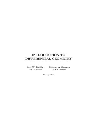
3Surface integrals3.1Parameterized SurfacesRecall that a parameterized curve is a C 1 function from an interval [a, b] R1 toR3 . If we replace the interval by subset of the plane R2 , we get a parameterizedsurface. Let’s look at a few of examples1) The upper half sphere of radius 1 centered at the origin can be parameterized using cartesian coordinates x u y vz 1 u2 v 2 2u v2 12) The upper half sphere can be parameterized using spherical coordinates x sin(φ) cos(θ) y sin(φ) sin(θ) z cos(φ) 0 φ π/2, 0 θ 2π(Since there is more than one convention, we should probably be clear aboutthis. For us, θ is the “polar” angle, and φ is the angle measured from the positvez-axis.)3) The upper half sphere can be parameterized using cylindrical coordinates x r cos(θ) y r sin(θ)z 1 r2 0 r 1, 0 θ 2πAn orientation on a curve is a choice of a direction for the curve. For asurface an orientation is a choice of “up” or “down”. The easist way to makethis precise is to view an orientation as a choice of (an upward, downward,outward or inward pointing) unit normal vector field n on S. A parameterizedsurface S x f (u, v) y g(u, v)z h(u, v) (u, v) Dis called smooth provided that f, g, h are C 1 , the function that they define fromD R3 is one to one, and the tangent vector fields x y zTu ,, u u u x y zTv ,, v v v18
are linearly independent. In this case, once we pick an ordering of the variables(say u first, v second) an orientation is determined by the normaln Tu Tv Tu Tv nTvTuSu constantv constantFIGURE 1If we look at the examples given earlier. (1) is smooth. However there isa slight problem with our examples (2) and (3). Here Tθ 0, when φ 0 inexample (2) and when r 0 in example (3). To deal with scenario, we willconsider a surface smooth if there is at least one smooth parameterization forit.Let C be a closed C 1 curve in R2 and D be the interior of C. D is an exampleof a surface with a boundary C. In this case the surface lies flat in the plane,but more general examples can be constructed by letting S be a parameterizedsurface x f (u, v) y g(u, v)z h(u, v) (u, v) D R2then the image of C in R3 will be the boundary of S. For example, the boundary19
of the upper half sphere S x sin(φ) cos(θ) y sin(φ) sin(θ)z cos(φ) 0 φ π/2, 0 θ 2πis the circle C given byx cos(θ), y sin(θ), z 0, 0 θ 2πIn what follows, we will need to match up the orientation of S and its boundarycurve. This will be done by the right hand rule: if the fingers of the right handpoint in the direction of C, then the direction of the thumb should be “up”.nSCFIGURE 23.2Surface IntegralsLet S be a smooth parameterized surface x f (u, v) y g(u, v)z h(u, v) (u, v) Dwith orientation corresponding to the ordering u, v. The symbols dx etc. canbe converted to the new coordinates as followsdx x xdu dv u v20
dy y ydu dv u v dx dy x x y y du dv du dv u v u v x y x y du dv u v v u (x, y) du dv (u, v)In this way, it is possible to convert any 2-form ω to uv-coordinates.DEFINITION 3.2.1 The integral of a 2-form on S is given by ZZZZ (x, y) (y, z) (z, x)F dx dy Gdy dz Hdz dx F G Hdudv (u, v) (u, v) (u, v)SDIn practice, the integral of a 2-form can be calculatedby first converting itRRto the form f (u, v)du dv, and then evaluating D f (u, v) dudv.Let S be the upper half sphere of radius 1 oriented with the upward normalparameterized using spherical coordinates, we getdx dy (x, y)dφ dθ cos(φ) sin(φ)dφ dθ (φ, θ)SoZZZ2ππ/2Zdx dy Scos(φ) sin(φ)dφdθ π00On the other hand if use the same surface parameterized using cylindricalcoordinates (x, y)dx dy dr dθ rdr dθ (r, θ)ThenZZZ2πZdx dy S1rdrdθ π00which leads to the same answer as one would hope. The general result is:THEOREM 3.2.2 Suppose that an oriented surface S has two different smoothC 1 parameterizations, then for any 2-form ω, the expression for the integrals ofω calculated with respect to both parameterizations agree.(This theorem needs to be applied to the half sphere with the point (0, 0, 1)removed in the above examples.) Let us give the proof. Suppose that u, vis a parameterization as above, and u p(s, t), v q(s, t) for one to one C 1 functions p, q on a domain E in pq-plane. We also want to assume that (u,v) (s,t) 0on E. This will ensure that s, t gives a new parameterization of S with the21
R2 is an expression F(x;y)dx G(x;y)dywhere F;Gare R-valued functions on the open set. A very important example of a di erential is given as follows: If f(x;y) is C1 R-valued function on an open set


![[MS-OFBA]: Office Forms Based Authentication Protocol](/img/3/ms-ofba.jpg)