Transcription
Differential Equations in RTutorial useR Conference Los Angeles 2014Karline Soetaert, & Thomas PetzoldtCentre for Estuarine and Marine Ecology (CEME)Royal Netherlands Institute for Sea Research (NIOZYerseke, The Netherlandskarline.soetaert@nioz.nlTechnische Universität DresdenFaculty of Environmental SciencesInstitute of Hydrobiology01062 -30
IntroModelsSolvPlotFitStateOutlineIHow to specify a modelIAn overview of solver functionsIPlotting, scenario comparison,IFitting models to data,ForcingDDEPDEDAECPUEnd
IntroModelsSolvPlotFitStateForcingOutlineIHow to specify a modelIAn overview of solver functionsIPlotting, scenario comparison,IFitting models to data,IForcing functions and eventsIPartial differential equations with ReacTranISpeeding upDDEPDEDAECPUEnd
Download R from the CRAN website: http://cran.r-project.org/DAECPUEnd
IntroModelsSolvPlotFitInstallingInstall a suitable editor. . . e.g. RStudioStateForcingDDEPDEDAECPUEnd
ingPackages can be installed from within R or Rstudio:. . . or via the command lineinstall.packages("deSolve", dependencies TRUE)CPUEnd
allingSeveral packages deal with differential equationsIdeSolve: main integration packageIrootSolve: steady-state solverIbvpSolve: boundary value problem solversIdeTestSet: ODE and DAE test set additional solversIReacTran: partial differential equationsIsimecol: interactive environment for implementing modelsAll packages have at least one author in common consistent interface.More, see CRAN Task View: Differential EquationsEnd
IntroModelsSolvPlotFitStateForcingDDEPDEGetting helpGetting help library(deSolve) ?deSolveIopens the main help page containingIIIIIIa short explanationa link to the main manual (vignette)“Solving Initial Value Differential Equations in R”links to additional manuals, papers and online resourcesreferencesa first exampleall our packages have such a ? packagename help file.DAECPUEnd
IntroModelsSolvPlotGetting help library(deSolve) example(deSolve)FitStateForcingDDEPDEDAECPUEnd
IntroModelsSolvPlotIntroductory exampleLet’s begin . . .Model specificationFitStateForcingDDEPDEDAECPUEnd
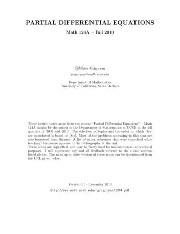
IntroModelsSolvPlotFitStateForcingIntroductory exampleLogistic growthDifferential equation dNN r ·N · 1 dtKAnalytical solutionNt KN0 e rtK N0 (e rt 1)R implementation logistic - function(t, r, K, N0) { K * N0 * exp(r * t) / (K N0 * (exp(r * t) - 1)) } plot(0:100, logistic(t 0:100, r 0.1, K 10, N0 0.1))DDEPDEDAECPUEnd
oductory exampleNumerical simulation in RWhy numerical solutions?INot all systems have an analytical solution,INumerical solutions allow discrete forcings, events, .Why R?IIf standard tool for statistics, why Prog for dynamic simulations?IThe community and the packages useR!2014End
ctory exampleNumerical solution of the logistic y(deSolve)model - function (time, y, parms) {with(as.list(c(y, parms)), {dN r * N * (1 - N / K)list(dN)})}yparmstimesDifferential equation„similar to formula on paper" - c(N 0.1) - c(r 0.1, K 10) - seq(0, 100, 1)out - ode(y, times, model, parms)plot(out)Numerical methods provided by thedeSolve packageCPUEnd
ntroductory exampleInspecting outputIPrint to screen head(out, n 187080.1345160Summary summary(out)NMin.0.1000001st Qu.1.096000Median5.999000Mean5.3960003rd ing plot(out, main "logistic growth", lwd 2)
ry example diagnostics(out)-------------------lsoda return code-------------------return code (idid) 2Integration was successful.-------------------INTEGER values-------------------123567891415The return code : 2The number of steps taken for the problem so far: 105The number of function evaluations for the problem so far: 211The method order last used (successfully): 5The order of the method to be attempted on the next step: 5If return flag -4,-5: the largest component in error vector 0The length of the real work array actually required: 36The length of the integer work array actually required: 21The number of Jacobian evaluations and LU decompositions so far: 0The method indicator for the last succesful step,1 adams (nonstiff), 2 bdf (stiff): 116 The current method indicator to be attempted on the next step,1 adams (nonstiff), 2 bdf (stiff): 1-------------------RSTATE valuesDAECPUEnd
IntroModelsSolvPlotFitStateForcingDDEPDEDAECoupled equationsCoupled ODEs: the rigidODE problemProblemIEuler equations of a rigid body without external forces.IThree dependent variables (y1 , y2 , y3 ), the coordinates of therotation vector,II1 , I2 , I3 are the principal moments of inertia.[3] E. Hairer, S. P. Norsett, and G Wanner. Solving Ordinary Differential Equations I: NonstiffProblems. Second Revised Edition. Springer-Verlag, Heidelberg, 2009CPUEnd
IntroModelsSolvPlotFitStateForcingCoupled equationsCoupled ODEs: the rigidODE equationsDifferential equationy10y20y30 (I2 I3 )/I1 · y2 y3 (I3 I1 )/I2 · y1 y3 (I1 I2 )/I3 · y1 y2ParametersI1 0.5, I2 2, I3 3Initial conditionsy1 (0) 1, y2 (0) 0, y3 (0) 0.9DDEPDEDAECPUEnd
IntroModelsSolvPlotFitStateForcingDDEPDECoupled equationsCoupled ODEs: the rigidODE problemR implementation library(deSolve)rigidode - function(t, y, parms) {dy1 - -2* y[2] * y[3]dy2 - 1.25 * y[1] * y[3]dy3 - -0.5 * y[1] * y[2]list(c(dy1, dy2, dy3))}yini - c(y1 1, y2 0, y3 0.9)times - seq(from 0, to 20, by 0.01)out - ode (times times, y yini, func rigidode, parms NULL) head (out, n 3)timey1y2y3[1,] 0.00 1.0000000 0.00000000 0.9000000[2,] 0.01 0.9998988 0.01124925 0.8999719[3,] 0.02 0.9995951 0.02249553 0.8998875DAECPUEnd
IntroModelsSolvPlotFitStateForcingDDEPDECoupled equationsCoupled ODEs: plotting the rigidODE problem plot(out)library(scatterplot3d)par(mar c(0, 0, 0, 0))scatterplot3d(out[,-1])DAECPUEnd
IntroModelsSolvPlotFitStateForcingDDEPDEDAECoupled equationsExerciseThe Rössler equationsy10y20y30 y2 y3 y1 a · y2 b y3 · (y1 c)Initial Conditionsy1 1, y2 1, y3 1Parametersa 0.2, b 0.2, c 5TasksISolve the ODEs on the interval [0, 100]IProduce a 3-D phase-plane plotIUse file examples/rigidODE.R.txt as a template[13] O.E. Rössler. An equation for continous chaos. Physics Letters A, 57 (5):397-398, 1976.CPUEnd
IntroModelsSolvPlotFitStateSolvers .Solver overview, stiffness, accuracyForcingDDEPDEDAECPUEnd
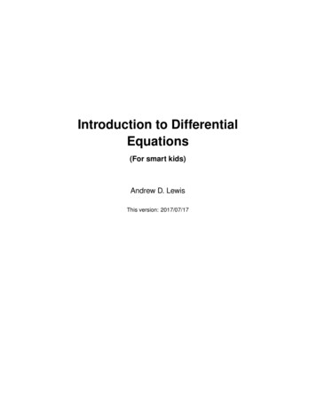
ration methods: package deSolve [22]EulerRunge KuttaExplicit RKLinear MultistepAdamsnon stiff problemsImplicit RKstiff problemsBDFPDEDAECPUEnd
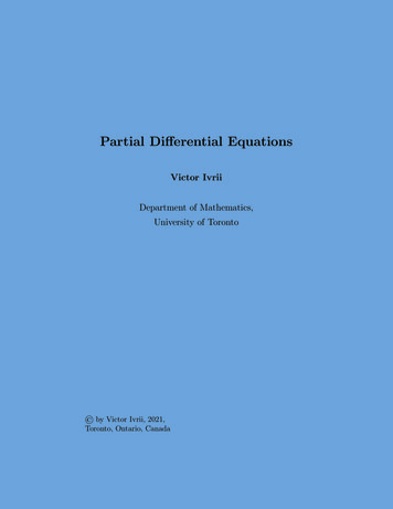
verviewbdf, adams, iterationreturns state at t dtsparse Jacobianbdf, adams, complex numbersDAE solverDAE; implicit RKeuler, ode23, ode45, rkMethodxxxxuser definedyesuser defineduser ngautoF(y’,t,y) 0Lags (DDE)lsodelsodesvodezvodedaspkradaurk, rk4, eulerEventsautomatic methodselectionRootslsoda/lsodarMy’ f(t,y)Notesy’ f(t,y)SolverstiffSolver overview: package deSolvexx- ode, ode.band, ode.1D, ode.2D, ode.3D: top level functions (wrappers)- red: functionality added by usadapted
tions of solver functionsTop level function ode(y, times, func, parms, method c("lsoda", "lsode", "lsodes", "lsodar", "vode", "daspk", "euler", "rk4", "ode23", "ode45", "radau", "bdf", "bdf d", "adams", "impAdams", "impAdams d", "iteration"), .)Workhorse function: the individual solver lsoda(y, times, func, parms, rtol 1e-6, atol 1e-6, jacfunc NULL, jactype "fullint", rootfunc NULL, verbose FALSE, nroot 0, tcrit NULL, hmin 0, hmax NULL, hini 0, ynames TRUE, maxordn 12, maxords 5, bandup NULL, banddown NULL, maxsteps 5000, dllname NULL, initfunc dllname, initpar parms, rpar NULL, ipar NULL, nout 0, outnames NULL, forcings NULL, initforc NULL, fcontrol NULL, events NULL, lags NULL,.)DAECPUEnd
viewArghhh, which solver and which options?Problem type?IODE: use ode,IDDE: use dede,IDAE: daspk or radau,IPDE: ode.1D, ode.2D, ode.3D,. . . others for specific purposes, e.g. root finding, difference equations (euler,iteration) or just to have a comprehensive solver suite (rk4, ode45).StiffnessIdefault solver lsoda selects method automatically,Iadams or bdf may speed up a little bit if degree of stiffness is known,Ivode or radau may help in difficult situations.End
ssSolvers for stiff systemsStiffnessIDifficult to give a precise definition. system where some components change more rapidly than others.Sometimes difficult to solve:Isolution can be numerically unstable,Imay require very small time steps (slow!),IdeSolve contains solvers that are suitable for stiff systems,But: “stiff solvers” slightly less efficient for “well behaving” systems.IGood news: lsoda selects automatically between stiff solver (bdf)and nonstiff method (adams).CPUEnd
ssVan der Pol equationOscillating behavior of electrical circuits containing tubes [24].2nd order ODEy 00 µ(1 y 2 )y 0 y 0. . . must be transformed into two 1st order equationsy10 y2y20 µ · (1 y1 2 ) · y2 y1IInitial values for state variables at t 0: y1(t 0) 2, y2(t 0) 0IOne parameter: µ large stiff system; µ small non-stiff.CPUEnd
ssModel implementation library(deSolve) vdpol - function (t, y, mu) { list(c( y[2], mu * (1 - y[1] 2) * y[2] - y[1] )) } yini - c(y1 2, y2 0) stiff - ode(y yini, func vdpol, times 0:3000, parms 1000) nonstiff - ode(y yini, func vdpol, times seq(0, 30, 0.01), parms 1) head(stiff, n -0.0006674088-0.0006677807-0.0006681535CPUEnd
fnessInteractive exerciseIThe following link opens in a web browser. It requires a recentversion of Firefox or Chrome, ideally in full-screen mode. Use Cursorkeys for slide transition:ILeft cursor guides you through the full presentation.IMouse and mouse wheel for full-screen panning and zoom.IPos1 brings you back to the first slide.IIexamples/vanderpol.svgThe following opens the code as text file for life demonstrations in RIexamples/vanderpol.R.txtEnd
fnessPlottingStiff solutionNonstiff solution plot(stiff, type "l", which "y1", lwd 2, ylab "y", main "IVP ODE, stiff") plot(nonstiff, type "l", which "y1", lwd 2, ylab "y", main "IVP ODE, nonstiff")End
Default solver, lsoda: system.time( stiff - ode(yini, 0:3000, vdpol, parms 1000) )user0.08system elapsed0.000.08 system.time( nonstiff - ode(yini, seq(0, 30, by 0.01), vdpol, parms 1) )user0.08system elapsed0.000.08Implicit solver, bdf: system.time( stiff - ode(yini, 0:3000, vdpol, parms 1000, )user0.06method "bdf")system elapsed0.000.07 system.time( nonstiff - ode(yini, seq(0, 30, by 0.01), vdpol, parms 1, method "bdf") )user0.05system elapsed0.000.04 Now use other solvers, e.g. adams, ode45, radau.
fnessResultsTiming results; your computer may be ison of solvers for a stiff and a non-stiff parametrisation of thevan der Pol equation (time in seconds, mean values of ten simulations onmy old AMD X2 3000 CPU).End
ssAccuracy and stabilityIOptions atol and rtol specify accuracy,IStability can be influenced by specifying hmax and maxsteps.CPUEnd
fnessAccuracy and stability - ctdatol (default 10 6 ) defines absolute threshold,I select appropriate value, depending of the size of yourstate variables,I may be between 10 300 (or even zero) and 10300 .rtol (default 10 6 ) defines relative threshold,I It makes no sense to specify values 10 15 becauseof the limited numerical resolution of double precisionarithmetics ( 16 digits).hmax is automatically set to the largest difference in times, toavoid that the simulation possibly ignores short-termevents. Sometimes, it may be set to a smaller value toimprove robustness of a simulation.hmin should normally not be changed.Example: Setting rtol and atol: examples/PCmod atol 0.R.txtEnd
, scenario comparison, observationsDDEPDEDAECPUEnd
wPlotting and printingMethods for plotting and extracting data in deSolveIsubset extracts specific variables that meet certain constraints.Iplot, hist create one plot per variable, in a number of panelsIimage for plotting 1-D, 2-D modelsIplot.1D and matplot.1D for plotting 1-D outputsI?plot.deSolve opens the main help filerootSolve has similar functionsIsubset extracts specific variables that meet certain constraints.Iplot for 1-D model outputs, image for plotting 2-D, 3-D modeloutputsI?plot.steady1D opens the main help fileCPUEnd
xamplesThe Lorenz equationsIchaotic dynamic system of ordinary differential equationsIthree variables, X , Y and Z represent idealized behavior of theearth’s atmosphere. chaos - function(t, state, parameters) {with(as.list(c(state)), {dx - -8/3 * x y * zdy - -10 * (y - z)dz - -x * y 28 * y - zlist(c(dx, dy, dz))})}yini - c(x 1, y 1, z 1)yini2 - yini c(1e-6, 0, 0)times - seq(0, 30, 0.01)out - ode(y yini, times times, func chaos, parms 0)out2 - ode(y yini2, times times, func chaos, parms 0)
sPlotting multiple scenariosIThe default for plotting one or more objects is a line plotIWe can plot as many objects of class deSolve as we wantBy default different outputs get different colors and line typesI plot(out, out2, lwd 2, lty 1)CPUEnd
sChanging the panel arrangementIDefault: Automatic number of panels per page up to 3 x 3IUse mfrow() or mfcol() to overrule plot(out, out2, lwd 2, lty 1, mfrow c(1, 3))IImportant: upon returning the default mfrow is NOT restored.CPUEnd
sPlotting styleIWe can change the style of the dataseries (col, lty, . . . )IIwill be effective for all figuresWe can change individual figure settings (title, labels, . . . )Ivector input can be specified by a list; NULL will select the default plot(out, out2, col c("blue", "orange"), main c("Xvalue", "Yvalue", "Zvalue"), xlim list(c(20, 30), c(25, 30), NULL), mfrow c(1, 3))CPUEnd
plesR’s default plot . . .is used if we extract single colums from the deSolve object plot(out[,"x"], out[,"y"], pch ".", main "Lorenz butterfly", xlab "x", ylab "y")End
xamplesUse deSolve’s subset . . . . . to select values that meet certain conditions XY - subset(out, select c("x", "y"), subset y 10 & x 40) plot(XY, main "Lorenz butterfly", xlab "x", ylab "y", pch ".")
xamplesPlotting multiple scenarios . . . . . is simple if number of outputs is known derivs - function(t, y, parms)with (as.list(parms), list(r * y * (1 - y/K)))times - seq(from 0, to 30, by 0.1)out - ode(y c(y 2), times, derivs, parms c(r 1, K 10))out2 - ode(y c(y 12), times, derivs, parms c(r 1, K 10))plot(out, out2, lwd 2)
xamplesPlotting multiple scenarios . . . . . with many or an unknown number of outputs in a list outlist - list()plist - cbind(r runif(30, min 0.1, max 5),K runif(30, min 8,max 15))for (i in 1:nrow(plist))outlist[[i]] - ode(y c(y 2), times, derivs, parms plist[i,])plot(out, outlist)
sObserved dataArguments obs and obspar are used to add observed data obs2 - data.frame(time c(1, 5, 10, 20, 25), y c(12, 10, 8, 9, 10)) plot(out, out2, obs obs2, obspar list(col "red", pch 18, cex 2))CPUEnd
plesObserved dataA list of observed data is allowed obs2 - data.frame(time c(1,5,10,20,25), y c(12,10,8,9,10)) obs1 - data.frame(time c(1,5,10,20,25), y c(1,6,8,9,10)) plot(out, out2, col c("blue", "red"), lwd 2, obs list(obs1, obs2), obspar list(col c("blue", "red"), pch 18, cex 2))End
IntroModelsSolvPlotFitOverviewFitting models to dataStateForcingDDEPDEDAECPUEnd
tting modelsGiven:Ia dynamic modelIdata for one or more state variablesWanted:Ia set of parameters that fits the dataApproach package FME:1. try an initial guess for the parameters2. define cost function (e.g. least squares) with modCost()3. fit the model with modFit4. plot model and dataDAECPUEnd
xample: Fit a compartment model to dataPharmacokinetic two compartment modelIa substance accumulated in the fat and eliminated by the liverItwo state variables, concentration in the fat CF and in the liver CLI3 parameters: transport (kFL , kLF ) and elimination (ke )dCL kFL CF kLF CL ke CLdtdCF kLF CL kFL CFdt library("FME") twocomp - function (time, y, parms, .) { with(as.list(c(parms, y)), { dCL - kFL * CF - kLF * CL - ke * CL # concentration in liver dCF kLF * CL - kFL * CF# concentration in fat list(c(dCL, dCF)) }) }
ple: Fit a compartment model to dataData and initial guess dat - data.frame(time seq(0, 28, 4),CL c(1.31, 0.61, 0.49, 0.41, 0.20, 0.12, 0.16, 0.21),CF c(1e-03, 0.041, 0.05, 0.039, 0.031, 0.025, 0.017, 0.012))parms - c(ke 0.2,kFL 0.1,kLF 0.05)times - seq(0, 40, length 200)y0 - c(CL 1, CF 0)out1 - ode(y0, times, twocomp, parms)plot(out1, obs dat)End
xample: Fit a compartment model to dataDefine cost function (least squares): cost - function(p) { out - ode(y0, times, twocomp, p) modCost(out, dat, weight "none") # try weight "std" or "mean" }Note:Inaming of oservation and simulation data must be identicalIdata may be given in cross table (wide) or data base format (long)Idifferent scaling and weighting optionsIoptional: sequential build-up of cost function
: Fit a compartment model to dataFit the model: parms - c(ke 0.2,kFL 0.1, fit - modFit(f cost, p parms) summary(fit)kLF 0.05)Parameters:Estimate Std. Error t value Pr( t )ke0.085460.012566.803 1.26e-05 ***kFL 0.672934.669530.1440.888kLF 0.069700.492690.1410.890--Signif. codes: 0 '***' 0.001 '**' 0.01 '*' 0.05 '.' 0.1 ' ' 1Residual standard error: 0.09723 on 13 degrees of freedomParameter correlation:kekFLkLFke 1.0000 0.4643 0.4554kFL 0.4643 1.0000 0.9932kLF 0.4554 0.9932 1.0000CPUEnd
: Fit a compartment model to dataCompare output with data out1 - ode(y0, times, twocomp, parms) out2 - ode(y0, times, twocomp, coef(fit)) plot(out1, out2, obs dat, obspar list(pch 16, col "red"))CPUEnd
xample: Fit a compartment model to dataFit parameters and initial values cost - function(p, data, .) { yy - p[c("CL", "CF")] pp - p[c("ke", "kFL", "kLF")] out - ode(yy, times, twocomp, pp) modCost(out, data, .) }Good start parameters can be very important: #parms - c(CL 1.2, CF 0.0,ke 0.2, kFL 0.1, kLF 0.05) parms - c(CL 1.2, CF 0.001, ke 0.2, kFL 0.1, kLF 0.05) fit - modFit(f cost, p parms, data dat, weight "std", lower rep(0, 5), upper c(2,2,1,1,1), method "Marq")
xample: Fit a compartment model to dataFit parameters and initial values y0 - coef(fit)[c("CL", "CF")]pp - coef(fit)[c("ke", "kFL", "kLF")]out3 - ode(y0, times, twocomp, pp)plot(out1, out2, out3, obs dat, col c("grey", "blue", "red"), lty 1)
IntroModelsSolvPlotFitStateForcingDDEPDEExample: Fit a compartment model to data summary(fit)Parameters:Estimate Std. Error t valueCL 1.2301394 0.0721467 17.051CF 0.0006821 0.00331180.206ke 0.1073348 0.01132319.479kFL 0.1770370 0.02893926.118kLF 0.0153857 0.00202897.583--Signif. codes: 0 '***' 0.001 '**'Pr( t 0.01 '*' 0.05 '.' 0.1 ' ' 1Residual standard error: 0.2032 on 11 degrees of freedomParameter correlation:CLCFkekFLkLFCL1.000000 0.003152 0.54175 -0.3837 -0.5494CF0.003152 1.000000 0.04449 -0.2229 -0.3529ke0.541751 0.044489 1.00000 -0.7083 -0.4287kFL -0.383735 -0.222888 -0.70830 1.0000 0.8340kLF -0.549433 -0.352886 -0.42874 0.8340 1.0000DAECPUEnd
IntroModelsSolvPlotFitStateSteady-stateSolver overview, 1-D, 2-D, 3-DForcingDDEPDEDAECPUEnd
ersTwo packages for Steady-state solutions:ReacTran: methods for numerical approximation of PDEsItran.1D(C, C.up, C.down, D, v, .)Itran.2D, tran.3DrootSolve: special solvers for rootsIsteady for 0-D modelsIsteady.1D, steady.2D, steady.3D for 1-D, 2-D, 3-D models[18] Soetaert, K. and Meysman, F. (2012) Reactive transport in aquatic ecosystems: Rapid model prototyping in the open source softwareR Environmental Modelling and Software 32, 49–60[21] Soetaert, K., Petzoldt, T. and Setzer, R. W. (2010 Solving Differential Equations in R The R Journal, 2010, 2, 5-15End
Steady-state Solver overview: package rootSolveSimple problems can be solved ate ODEs by Newton-Raphson method, full orbanded Jacobiansteady-state ODEs by Newton-Raphson method, arbitrary sparse JacobianOthers are solved by dynamically running to steady-statemethod "runsteady") for 0-D modelsIsteady( .Isteady.1D( .Ino special solver for higher dimensions - but use ode.2D, ode.3Dfrom deSolve for sufficiently long time(adapted from [21])method "runsteady") for 1-D modelsCPUEnd
Options of solver functionsTop level function steady(y, time NULL, func, parms, method "stode", .)Workhorse function: the individual solver stode(y, time 0, func, parms NULL, rtol 1e-06, atol 1e-08, ctol 1e-08, jacfunc NULL, jactype "fullint", verbose FALSE, bandup 1, banddown 1, positive FALSE, maxiter 100, ynames TRUE, dllname NULL, initfunc dllname, initpar parms, rpar NULL, ipar NULL, nout 0, outnames NULL, forcings NULL, initforc NULL, fcontrol NULL, .)NotesIpositive TRUE forces to find relevant solutions for quantititiesthat can not be negative.Iynames can be used to label the output – useful for plottingCPUEnd
s1-D problem: polluted estuaryProblem formulationAmmonia and oxygen are described in an estuary. They react to formnitrate. The concentrations are at steady state.00rnit 3 x(D NH x ) O2 x (D x )2 r · NH3 · OO2 k3 v NH x O2 v x rnit2rnit p · (O2 s O2 )Iparameters: k 1, r 0.1, p 0.1, O2 s 300, v 1000, D 1e 7IThe estuary is 100 km long.IThe boundary conditions are:NH3 (0) 500, O2 (0) 50, NH3 (1e 5 ) 10, O2 (1e 5 ) 30CPUEnd
lluted estuary in Rdefine grid: require(ReacTran) N - 1000 Grid - setup.grid.1D(N N, L 100000)derivative function: Estuary - function(t, y, parms) { NH3 - y[1:N] O2 - y[(N 1):(2*N)] tranNH3 - tran.1D (C NH3, D 1e7, v 1000, C.up 500, C.down 10, dx Grid) dC tranO2 - tran.1D (C O2 , D 1e7, v 1000, C.up 100, C.down 250, dx Grid) dC r nit - 0.1 * O2 / (O2 1) * NH3 dNH3 - tranNH3 - r nit dO2 - tranO2 - 2 * r nit 0.1 * (300 - O2) list(c( dNH3, dO2 ), r nit r nit) }numerical solution: print(system.time( std - steady.1D(y runif(2 * N), parms NULL, names c("NH3", "O2"), func Estuary, dimens N, positive TRUE)))user0.10system elapsed0.000.09DAECPUEnd
IntroModelsSolvPlotFitStateForcingExamplesPlotting plot(std, which c("NH3", "O2", "r nit"), lwd 2, mfrow c(1,3), grid Grid x.mid, xlab "distance, m", ylab c("mmol m-3", "mmol m-3", "mmol m-3 d-1"))DDEPDEDAECPUEnd
otting with Observations obs - data.frame(x seq(0, 9e4, by 1e4), O2 c(100, 0, 0, 100, 150, 200, 250, 300, 300, 300)) plot(std, which c("NH3", "O2", "r nit"), lwd 2, obs obs, obspar list(pch 18, col "red", cex 2), grid Grid x.mid, xlab "distance, m", ylab c("mmol m-3", "mmol m-3", "mmol m-3 d-1"), mfrow c(1,3))DAECPUEnd
plesSteady-state of a 2-D PDEProblem formulationA relatively stiff PDE is the combustion problem, describing diffusion andreaction in a 2-dimensional domain (from [6]). The steady-state problemis:R0 · ( K U) (1 α U) exp(δ(1 1/U))αδIThe domain is rectangular ([0,1]*[0,1])IK 1, α 1, δ 20, R 5,IDownstream boundary is prescribed as a known value (1)IUpstream boundary: zero-fluxEnd
s2-D combustion problem in Rgrid and parameters: library(ReacTran)N - 100Grid - setup.grid.1D(0, 1, N N)alfa - 1; delta - 20; R - 5derivative function: Combustion - function(t, y, p) { U - matrix(nrow N, ncol N, data y) reac - R /alfa/delta * (1 alfa-U) * exp(delta*(1-1/U)) tran - tran.2D(C U, D.x 1, flux.x.up 0, flux.y.up 0, C.x.down 1, C.y.down 1, dx Grid, dy Grid) list (tran dC reac) }solution (10000 equations): print(system.time( std - steady.2D(y rep(1, N*N), parms NULL, func Combustion, nspec 1, dimens c(N, N), lrw 1e6, positive TRUE) ))user1.52system elapsed0.001.52CPUEnd
IntroModelsSolvPlotFitStateForcingExamplesPlotting image(std, main "Combustion", legend TRUE)DDEPDEDAECPUEnd
sSteady-state of a 3-D PDEProblem formulation3-D problems are computationally heavy - only smaller problems can besolved in RModel of diffusion and simple reaction in a 3-dimensional domain.0 · ( D Y ) r YIThe domain is rectangular ([0, 1] [0, 1] [0, 1])ID 1, r 0.025,IInitial condition: constant: U(x, y , 0) 1.IUpstream and Downstream boundaries: 1CPUEnd
D problem in Rgrid and parameters: library(ReacTran) n - 20 Grid - setup.grid.1D(0, 1, N n)derivative function: diffusion3D - function(t, Y, par) { yy - array(dim c(n, n, n), data Y) # vector to 3-D array dY - -0.025 * yy# consumption BND - matrix(nrow n, ncol n, 1)# boundary concentration dY - dY tran.3D(C yy, C.x.up BND, C.y.up BND, C.z.up BND, C.x.down BND, C.y.down BND, C.z.down BND, D.x 1, D.y 1, D.z 1, dx Grid, dy Grid, dz Grid) dC return(list(dY)) }solution (10000 equations): print(system.time( ST3 - steady.3D(y rep(1, n*n*n), func diffusion3D, parms NULL, pos TRUE, dimens c(n, n, n), lrw 2000000) ))user2.01system elapsed0.012.03DAECPUEnd
inga selection of 2-D projections, in the x-direction image(ST3, mfrow c(2, 2), add.contour TRUE, legend TRUE, dimselect list(x c(4, 8, 12, 16)))PDEDAECPUEnd
IntroModelsSolvPlotFitStateForcingUnder control: Forcing functions and eventsDDEPDEDAECPUEnd
inuities in dynamic modelsMost solvers assume that dynamics is smoothHowever, there can be several types of discontinuities:INon-smooth external variablesIDiscontinuities in the derivativesIDiscontinuites in the values of the state variablesA solver does not have large problems with first two types ofdiscontinuities, but changing the values of state variables is much moredifficult.CPUEnd
l VariablesExternal variables in dynamic models. . . also called forcing functionsWhy external variables?ISome important phenomena are not explicitly included in adifferential equation model, but imposed as a time series. (e.g.sunlight, important for plant growth is never “modeled”).ISomehow, during the integration, the model needs to know thevalue of the external variable at each time step!CPUEnd
rnal VariablesExternal variables in dynamic modelsImplementation in RIIR has an ingenious function that is especially suited for this task:function approxfunIt is used in two steps:IFirst an interpolating function is constructed, that contains the data.This is done before solving the differential equation.afun - approxfun(data)IWithin the derivative function, this interpolating function is called toprovide the interpolated value at the requested time point (
Intro Models Solv Plot Fit State Forcing DDE PDE DAE CPU End Installing Several packages deal with di erential equations I deSolve: main integration package I rootSolve: steady-state solver I bvpSolve: boundary value problem solvers I deTestSet: ODE and DAE test set additional solvers I ReacTran: partial di erential equations I simecol: interactive environment for implementing models