Transcription
Differential Geometry in PhysicsGabriel LugoUniversity of North Carolina Wilmington
iThis book is dedicated to my family, for without their love and support, this work would have not beenpossible. Most importantly, let us not forget that our greatest gift are our children and our children’schildren, who stand as a reminder, that curiosity and imagination is what drives our intellectual pursuits,detaching us from the mundane and confinement to Earthly values, and bringing us closer to the divine andthe infinite.The 1992 edition of this document was reproduced and assigned an ISBN code, by the Printing services of theUniversity of North Carolina Wilmington, from a camera-ready copy supplied by the author. Thereafter, thedocument has been made available for free download as the main text for the Differential Geometry courseoffered in this department. The text was generated on a desktop computer using LATEX. 1992,1998, 2006, 2020, 2021Escher detail above from “Belvedere” plate 230, [?].All other figures and illustrations were produced by the author or taken from photographs taken by theauthor and family members. Exceptions are included with appropriate attribution.All rights reserved. No part of this publication may be reproduced, stored in a retrieval system, or transmitted, in any form or by any means, electronic, mechanical, photocopying, recording or otherwise, withoutthe written permission of the author. Printed in the United States of America.
ii
PrefaceThese notes were developed as part a course on differential geometry at the advanced undergraduate,first year graduate level, which the author has taught for several years. There are many excellent texts indifferential geometry but very few have an early introduction to differential forms and their applications toPhysics. It is purpose of these notes to:1. Provide a bridge between the very practical formulation of classical differential geometry created byearly masters of the late 1800’s, and the more elegant but less intuitive modern formulation in termsof manifolds, bundles and differential forms. In particular, the central topic of curvature is presentedin three different but equivalent formalisms.2. Present the subject of differential geometry with an emphasis on making the material readable tophysicists who may have encountered some of the concepts in the context of classical or quantummechanics, but wish to strengthen the rigor of the mathematics. A source of inspiration for this goal isrooted in the shock to this author as a graduate student in the 70’s at Berkeley, at observing the gaspingfailure of communications between the particle physicists working on gauge theories and differentialgeometers working on connection on fiber bundles. They seemed to be completely unaware at the time,that they were working on the same subject.3. Make the material as readable as possible for those who stand at the boundary between theoreticalphysics and applied mathematics. For this reason, it will be occasionally necessary to sacrifice somemathematical rigor or depth of physics, in favor of ease of comprehension.4. Provide the formal geometrical background which constitute the foundation of the mathematical theoryof general relativity.5. Introduce examples of other applications of differential geometry to physics that might not appear intraditional texts used in courses for mathematics students.This book should be accessible to students who have completed traditional training in advanced calculus,linear algebra, and differential equations. Students who master the entirety of this material will have gainedinsight in a very powerful tool in mathematical physics at the graduate level.Gabriel Lugo, Ph. D.Mathematical Sciences and StatisticsUNCWWilmington, NC 28403lugo@uncw.eduiii
iv
ContentsPrefaceiii1 Vectors and Curves1.1 Tangent Vectors . . . . . . . . .1.2 Differentiable Maps . . . . . . . .1.3 Curves in R3 . . . . . . . . . . .1.3.1 Parametric Curves . . . .1.3.2 Velocity . . . . . . . . . .1.3.3 Frenet Frames . . . . . .1.4 Fundamental Theorem of Curves1.4.1 Isometries . . . . . . . . .1.4.2 Natural Equations . . . .1168810121719222 Differential Forms2.1 One-Forms . . . . . . . . . . . . . .2.2 Tensors . . . . . . . . . . . . . . . .2.2.1 Tensor Products . . . . . . .2.2.2 Inner Product . . . . . . . . .2.2.3 Minkowski Space . . . . . . .2.2.4 Wedge Products and 2-Forms2.2.5 Determinants . . . . . . . .2.2.6 Vector Identities . . . . . . .2.2.7 n-Forms . . . . . . . . . . .2.3 Exterior Derivatives . . . . . . . . .2.3.1 Pull-back . . . . . . . . . . .2.3.2 Stokes’ Theorem in Rn . . .2.4 The Hodge ? Operator . . . . . . . .2.4.1 Dual Forms . . . . . . . . . .2.4.2 Laplacian . . . . . . . . . . .2.4.3 Maxwell Equations . . . . . .27272929303334373941424448515155563 Connections3.1 Frames . . . . . . . . . .3.2 Curvilinear Coordinates3.3 Covariant Derivative . .3.4 Cartan Equations . . . .61616366704 Theory of Surfaces4.1 Manifolds . . . . . . . . . . . . . . . . . .4.2 The First Fundamental Form . . . . . . .4.3 The Second Fundamental Form . . . . . .4.4 Curvature . . . . . . . . . . . . . . . . . .4.4.1 Classical Formulation of Curvature.757578858989.v
0CONTENTS4.54.4.2 Covariant Derivative Formulation of CurvatureFundamental Equations . . . . . . . . . . . . . . . . .4.5.1 Gauss-Weingarten Equations . . . . . . . . . .4.5.2 Curvature Tensor, Gauss’s Theorema Egregium. 91. 95. 95. 1015 Geometry of Surfaces5.1 Surfaces of Constant Curvature . . . . . . . . . .5.1.1 Ruled and Developable Surfaces . . . . .5.1.2 Surfaces of Constant Positive Curvature .5.1.3 Surfaces of Constant Negative Curvature5.1.4 Bäcklund Transforms . . . . . . . . . . .5.2 Minimal Surfaces . . . . . . . . . . . . . . . . . .5.2.1 Minimal Area Property . . . . . . . . . .5.2.2 Conformal Mappings . . . . . . . . . . . .5.2.3 Isothermal Coordinates . . . . . . . . . .5.2.4 Stereographic Projection . . . . . . . . . .5.2.5 Minimal Surfaces by Conformal Maps . .1091091091091091091091091091091091096 Riemannian Geometry6.1 Riemannian Manifolds . . . . . . . .6.2 Submanifolds . . . . . . . . . . . . .6.3 Sectional Curvature . . . . . . . . .6.4 Big D . . . . . . . . . . . . . . . . .6.4.1 Linear Connections . . . . . .6.4.2 Affine Connections . . . . . .6.4.3 Exterior Covariant Derivative6.4.4 Parallelism . . . . . . . . . .6.5 Lorentzian Manifolds . . . . . . . . .6.6 Geodesics . . . . . . . . . . . . . . .6.7 Geodesics in GR . . . . . . . . . . .6.8 Gauss-Bonnet Theorem . . . . . . s147Index148
Chapter 1Vectors and Curves1.1Tangent Vectors1.1.1 Definition Euclidean n-space Rn is defined as the set of ordered n-tuples p(p1, . . . , pn), where pi R,for each i 1, . . . , n. We may associate a position vector p (p1, . . . , pn) with any given point p in n-space.Given any two n-tuples p (p1, . . . , pn), q (q1, . . . , qn) and any real number c, we define two operations:p q (p1 q 1 , . . . , pn q n ),c p (c p1 , . . . , c pn ).(1.1)These two operations of vector sum and multiplication by a scalar satisfy all the 8 properties needed to givethe set V Rn a natural structure of a vector space. It is common to use the same notation Rn for thespace of n-tuples and for the vector space of position vectors. Technically we should write p Rn whenthink of Rn as a metric space and p Rn when we think of it as vector space, but as most authors, we willfreely abuse the notation.11.1.2Definition Let xi be the real valued functions in Rn such thatxi (p) pifor any point p (p1 , . . . , pn ). The functions xi are then called the natural coordinate functions. Whenconvenient, we revert to the usual names for the coordinates, x1 x, x2 y and x3 z in R3 . A smallawkwardness might occur in the transition to modern notation. In classical vector calculus, a point in Rn isoften denoted by x, in which case, we pick up the coordinates with the slot projection functions ui : Rn Rdefined byui (x) xi .1.1.3 Definition A real valued function in Rn is of class C r if all the partial derivatives of the function upto order r exist and are continuous. The space of infinitely differentiable (smooth) functions will be denotedby C (Rn ) or F (Rn ).1 Inthese notes we will use the following index conventions: In Rn , indices such as i, j, k, l, m, n, run from 1 to n. In space-time, indices such as µ, ν, ρ, σ, run from 0 to 3. On surfaces in R3 , indices such as α, β, γ, δ, run from 1 to 2. Spinor indices such as A, B, Ȧ, Ḃ run from 1 to 2.1
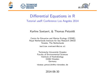
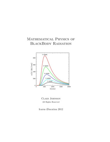
2CHAPTER 1. VECTORS AND CURVES1.1.4 Definition Let V and V 0 be finite dimensional vector spaces such as V Rk and V 0 Rn , andlet L(V, V 0 ) be the space of linear transformations from V to V 0 . The set of linear functionals L(V, R) iscalled the dual vector space V . This space has the same dimension as V .In calculus, vectors are usually regarded as arrows characterized by a direction and a length. Thus,vectors are considered as independent of their location in space. Because of physical and mathematicalreasons, it is advantageous to introduce a notion of vectors that does depend on location. For example, ifthe vector is to represent a force acting on a rigid body, then the resulting equations of motion will obviouslydepend on the point at which the force is applied. In later chapters, we will consider vectors on curvedspaces; in these cases, the positions of the vectors are crucial. For instance, a unit vector pointing north atthe earth’s equator is not at all the same as a unit vector pointing north at the tropic of Capricorn. Thisexample should help motivate the following definition.1.1.5 Definition A tangent vector Xp in Rn , is an ordered pair {x, p}. We may regard x as an ordinaryadvanced calculus “arrow-vector” and p is the position vector of the foot of the arrow.The collection of all tangent vectors at a point p Rn is called the tangent space at p and will bedenoted by Tp (Rn ). Given two tangent vectors Xp , Yp and a constant c, we can define new tangent vectorsat p by (X Y )p Xp Yp and (cX)p cXp . With this definition, it is clear that for each point p, thecorresponding tangent space Tp (Rn ) at that point has the structure of a vector space. On the other hand,there is no natural way to add two tangent vectors at different points.The set T (Rn ) (or simply T Rn ) consisting of the union of all tangent spaces at all points in Rn is calledthe tangent bundle. This object is not a vector space, but as we will see later it has much more structurethan just a set.Fig. 1.1: Tangent Bundle1.1.6 Definition A vector field X in U Rn is a section of the tangent bundle, that is, a smooth functionfrom U to T (U ). The space of sections Γ(T (U ) is also denoted by X (U ).The difference between a tangent vector and a vector field is that inthe latter case, the coefficients v i of x are smooth functions of xi . Since ingeneral there are not enough dimensions to depict a tangent bundle andvector fields as sections thereof, we use abstract diagrams such as shownFigure 1.1. In such a picture, the base space M (in this case M Rn )is compressed into the continuum at the bottom of the picture in whichseveral points p1 , . . . , pk are shown. To each such point one attaches atangent space. Here, the tangent spaces are just copies of Rn shown asvertical “fibers” in the diagram. The vector component xp of a tangentvector at the point p is depicted as an arrow embedded in the fiber.The union of all such fibers constitutes the tangent bundle T M T Rn .A section of the bundle amounts to assigning a tangent vector to everyFig. 1.2: Vector Fieldpoint in the base. It is required that such assignment of vectors is donein a smooth way so that there are no major “changes” of the vector fieldbetween nearby points.Given any two vector fields X and Y and any smooth function f , we can define new vector fields X Y
1.1. TANGENT VECTORS3and f X by(X Y )p Xp Yp(f X)p f Xp ,(1.2)so that X (U ) has the structure of a vector space over R. The subscript notation Xp indicating the locationof a tangent vector is sometimes cumbersome, but necessary to distinguish them from vector fields.Vector fields are essential objects in physical applications. If we consider the flow of a fluid in a region,the velocity vector field represents the speed and direction of the flow of the fluid at that point. Otherexamples of vector fields in classical physics are the electric, magnetic, and gravitational fields. The vectorfield in figure 1.2 represents a magnetic field around an electrical wire pointing out of the page.1.1.7 Definition Let Xp {x, p} be a tangent vector in an open neighborhood U of a point p Rn andlet f be a C function in U . The directional derivative of f at the point p, in the direction of x, is definedbyXp (f ) f (p) · x,(1.3)where f (p) is the gradient of the function f at the point p. The notationXp (f ) Xp f,is also commonly used. This notation emphasizes that, in differential geometry, we may think of a tangentvector at a point as an operator on the space of smooth functions in a neighborhood of the point. Theoperator assigns to a function f , the directional derivative of that function in the direction of the vector.Here we need not assume as in calculus that the direction vectors have unit length.It is easy to generalize the notion of directional derivatives to vector fields by definingX(f ) X f f · x,(1.4)nwhere the function f and the components of x depend smoothly on the points of R .The tangent space at a point p in Rn can be envisioned as another copy of Rn superimposed at thepoint p. Thus, at a point p in R2 , the tangent space consist of the point p and a copy of the vector space R2attached as a “tangent plane” at the point p. Since the base space is a flat 2-dimensional continuum, thetangent plane for each point appears indistinguishable from the base space as in figure 1.2.Later we will define the tangent space for a curved continuum such as a surface in R3 as shown in figure1.3. In this case, the tangent space at a point p consists of the vector space of all vectors actually tangentto the surface at the given point.Fig. 1.3: Tangent vectors Xp , Yp on a surface in R3 .1.1.8Proposition If f, g F (Rn ), a, b R, and X X (Rn ) is a vector field, thenX(af bg) aX(f ) bX(g),X(f g) f X(g) gX(f ).(1.5)
4CHAPTER 1. VECTORS AND CURVES1.1.9 Remark The space of smooth functions is a ring, ignoring a small technicality with domains. Anoperator such as a vector field with the properties above, is called a linear derivation on F (Rn ). ProofFirst, let us develop an mathematical expression for tangent vectors and vector fields that will facilitatecomputation.Let p U be a point and let xi be the coordinate functions in U . Suppose that Xp {x, p}, where thecomponents of the Euclidean vector x are (v 1 , . . . , v n ). Then, for any function f , the tangent vector Xpoperates on f according to the formula nX f(p).(1.6)Xp (f ) vi xii 1It is therefore natural to identify the tangent vector Xp with the differential operatorXp nXvi i 1Xp v1 xi x1 (1.7)p · · · vnp xn .pNotation: We will be using Einstein’s convention to suppress the summation symbol whenever an expressioncontains a repeated index. Thus, for example, the equation above could be simply written as .(1.8)Xp v i xi pThis equation implies that the action of the vector Xp on the coordinate functions xi yields the componentsv i of the vector. In elementary treatments, vectors are often identified with the components of the vector,and this may cause some confusion.The operators( ) {e1 , . . . , ek } p ,., x1 p xn pform a basis for the tangent space Tp (Rn ) at the point p, and any tangent vector can be written as alinear combination of these basis vectors. The quantities v i are called the contravariant components of thetangent vector. Thus, for example, the Euclidean vector in R3x 3i 4j 3klocated at a point p, would correspond to the tangent vector Xp 3 4 3. x p y p z pLet X v i be an arbitrary vector field and let f and g be real-valued functions. Then xiX(af bg) (af bg) xi v i i (af ) v i i (bg) x xi fi gav bv xi xiaX(f ) bX(g).vi
1.1. TANGENT VECTORS5Similarly,X(f g) (f g) xi v i f i (g) v i g i (f ) x x g ff v i i gv i i x xf X(g) gX(f ).viTo re-emphasize, any quantity in Euclidean space which satisfies relations 1.5 is a called a linear derivationon the space of smooth functions. The word linear here is used in the usual sense of a linear operator inlinear algebra, and the word derivation means that the operator satisfies Leibnitz’ rule.The proof of the following proposition is slightly beyond the scope of this course, but the proposition isimportant because it characterizes vector fields in a coordinate-independent manner.1.1.10 Proposition Any linear derivation on F (Rn ) is a vector field.This result allows us to identify vector fields with linear derivations. This step is a big departure from theusual concept of a “calculus” vector. To a differential geometer, a vector is a linear operator whose inputsare functions and whose output are functions that at each point represent the directional derivative in thedirection of the Euclidean vector.1.1.11 Example Given the point p(1, 1), the Euclidean vector x (3, 4), and the function f (x, y) x2 y 2 , we associate x with the tangent vectorXp 3 4 . x yThen, Xp (f )1.1.12 3 f x 4p f y 3(2x) p 4(2y) p , 3(2) 4(2) 14. ,pExample Let f (x, y, z) xy 2 z 3 and x (3x, 2y, z). Then X(f ) f x 2y f y z f z 3x 3x(y 2 z 3 ) 2y(2xyz 3 ) z(3xy 2 z 2 ), 3xy 2 z 3 4xy 2 z 3 3xy 2 z 3 10xy 2 z 3 .1.1.13 Definition Let X be a vector field in Rn and p be a point. A curve α(t) with α(0) p is calledan integral curve of X if α0 (0) Xp , and, whenever α(t) is the domain of the vector field, α0 (t) Xα(t) .In elementary calculus and differential equations, the families of integral curves of a vector field are calledthe streamlines, suggesting the trajectories of a fluid with velocity vector X. In figure 1.2, the integral curveswould be circles that fit neatly along the flow of the vector field. In local coordinates, the expression definingintegral curves of X constitutes a system of first order differential equations, so the existence and uniquenessof solutions apply locally. We will treat this in more detail in section ?
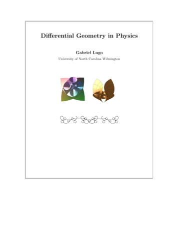
6CHAPTER 1. VECTORS AND CURVES1.2Differentiable Maps1.2.1 Definition Let F : Rn Rm be a vector function defined by coordinate entries F (p) (f 1 (p), f 2 (p), . . . f m (p)). The vector function is called a mapping if the coordinate functions are all differentiable. If the coordinate functions are C , F is called a smooth mapping. If (x1 , x2 , . . . xn ) are localcoordinates in Rn and (y 1 , y 2 , . . . y m ) local coordinates in Rm , a map y F (x) is represented in advancedcalculus by m functions of n variablesy j f j (xi ),i 1. . . . n, j 1.m.(1.9)A map F : Rn Rm is differentiable at a point p Rn if there exists a linear transformation DF (p :Rn ) Rm such that F (p h) F (p) DF (p)(h) lim 0(1.10)h 0 h The linear transformation DF (p)is called the Jacobian. A differentiable map that is invertible and theinverse is differentiable, is called a diffeomorphism.Remarks1. A differentiable mapping F : I R Rn is what we called a curve. If t I [a, b], the mappinggives a parametrization x(t), as we discussed in the previous section.2. A differentiable mapping F : R Rn Rn is called a coordinate transformation. Thus, for example,the mapping F : (u, v) R2 (x, y) R2 , given by functions x x(u, v), y y(u, v), wouldconstitute a change of coordinates from (u, v) to (x, y). The most familiar case is the polar coordinatestransformation x r cos θ, y r sin θ.3. A differentiable mapping F : R R2 R3 is what in calculus we called a parametric surface. Typically, one assumes that R is a simple closed region, such as a rectangle. If one denotes the coordinatesin R2 by (u, v) R, and x R3 , the parametrization is written as x(u, v) (x(u, v), y(u, v), z(u, v)).The treatment of surfaces in R3 is presented in chapter 4. If R3 is replaced by Rn , the mapping locallyrepresents a 2-dimensional surface in a space of n dimensions.For each point p Rn , we say that the Jacobian induces a linear transformation F from the tangentspace Tp Rn to the tangent space TF (p) Rm . In differential geometry we this Jacobian map is also called thepush-forward. If we let X be a tangent vector in Rn , then the tangent vector F X in Rm is defined byF X(f ) X(f F ),(1.11)where f F (Rm ). (See figure 1.4)Fig. 1.4: Jacobian Map.As shown in the diagram, F X(f ) is evaluated at F (p) whereas X is evaluated at p. So, to be precise,equation 1.11 should really be written asF X(f )(F (p)) X(f F )(p),(1.12)F X(f ) F X(f F ),(1.13)As we have learned from linear algebra, to find a matrix representation of a linear map in a particular basis, one applies the map to the basis vectors. If we denote by { xi } the basis for the tangent space at a point
1.2. DIFFERENTIABLE MAPS7p Rn and by { y j } the basis for the tangent space at the corresponding point F (p) Rm with coordinatesgiven by y j f j (xi ), the push-forward definition reads, )(f ) (f F ), xi xi f y j , y j xi y j F ( i ) . x xi y jF (In other words, the matrix representation of F in standard basis is in fact the Jacobian matrix. In classicalnotation, we simply write the Jacobian map in the familiar form, y j .i x xi y j(1.14)1.2.2 Theorem If F : Rn Rm and G : Rm Rp are mappings, then (G F ) G F .Proof Let X Tp (R)n , and f be a smooth function f : Rp R. Then,(G F ) (X)(f ) X(f (G F ), X((f G) F ), F (X)(f G), G (F (X)(f )), (G F )(X)(f ).1.2.3 Inverse Function Theorem. When m n, mappings are called change of coordinates. In theterminology of tangent spaces, the classical inverse function theorem states that if the Jacobian map F is a vector space isomorphism at a point, then there exists a neighborhood of the point in which F is adiffeomorphism.1.2.4Remarks1. Equation 1.14 shows that under change of coordinates, basis tangent vectors and by linearity all tangentvectors transform by multiplication by the matrix representation of the Jacobian. This is the sourceof the almost tautological definition in physics, that a contravariant tensor of rank one, is one thattransforms like a contravariant tensor of rank one.2. Many authors use the notation dF to denote the push-forward map F .3. If F : Rn Rm and G : Rm Rp are mappings, we leave it as an exercise for the reader to verifythat the formula (G F ) G F for the composition of linear transformations corresponds to theclassical chain rule.4. As we will see later, the concept of the push-forward extends to manifold mappings F : M N .
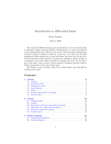
81.31.3.1CHAPTER 1. VECTORS AND CURVESCurves in R3Parametric Curves1.3.1 Definition A curve α(t) in R3 is a C map from an interval I R into R3 . The curve assigns toeach value of a parameter t R, a point (α1 (t), α2 (t), α3 (t)) R3 .αI R7 R3t7 α(t) (α1 (t), α2 (t), α3 (t))One may think of the parameter t as representing time, and the curve α as representing the trajectory of amoving point particle as a function of time. When convenient, we also use classical notation for the positionvectorx(t) (x1 (t), x2 (t), x3 (t)),(1.15)which is more prevalent in vector calculus and elementary physics textbooks. Of course, what this notationreally means isxi (t) (ui α)(t),(1.16)where ui are the coordinate slot functions in an open set in R31.3.2Example Letα(t) (a1 t b1 , a2 t b2 , a3 t b3 ).(1.17)This equation represents a straight line passing through the point p (b1 , b2 , b3 ), in the direction of thevector v (a1 , a2 , a3 ).1.3.3Example Letα(t) (a cos ωt, a sin ωt, bt).(1.18)This curve is called a circular helix. Geometrically, we may view the curve as the path described by thehypotenuse of a triangle with slope b, which is wrapped around a circular cylinder of radius a. The projectionof the helix onto the xy-plane is a circle and the curve rises at a constant rate in the z-direction (See Figure1.5a). Similarly, The equation α(t) (a cosh ωt, a sinh ωt, bt) is called a hyperbolic ”helix.” It represents thegraph of curve that wraps around a hyperbolic cylinder rising at a constant rate.Fig. 1.5: a) Circular Helix. b) Temple of Viviani1.3.4Example Letα(t) (a(1 cos t), a sin t, 2a sin(t/2)).(1.19)
1.3. CURVES IN R39This curve is called the Temple of Viviani. Geometrically, this is the curve of intersection of a spherex2 y 2 z 2 4a2 of radius 2a, and the cylinder x2 y 2 2ax of radius a, with a generator tangent to thediameter of the sphere along the z-axis (See Figure 1.5b).The Temple of Viviani is of historical interest in the development of calculus. The problem was posedanonymously by Viviani to Leibnitz, to determine on the surface of a semi-sphere, four identical windows,in such a way that the remaining surface be equivalent to a square. It appears as if Viviani was challengingthe effectiveness of the new methods of calculus against the power of traditional geometry.It is said that Leibnitz understood the nature of the challengeand solved the problem in one day. Not knowing the proposer ofthe enigma, he sent the solution to his Serenity Ferdinando, as heguessed that the challenge must have originated from prominent Italian mathematicians. Upon receipt of the solution by Leibnitz, Viviani posted a mechanical solution without proof. He described it asusing a boring device to remove from a semisphere, the surface areacut by two cylinders with half the radius, and which are tangentialto a diameter of the base. Upon realizing this could not physicallybe rendered as a temple since the roof surface would rest on onlyfour points, Viviani no longer spoke of a temple but referred to theshape as a “sail.”1.3.5 Definition Let α : I R3 be a curve in R3 given in components as above α (α1 , α2 , α3 ). Foreach point t I we define the velocity or tangent vector of the curve by 1dα dα2 dα3,,.(1.20)α0 (t) dt dt dt α(t)At each point of the curve, the velocity vector is tangent to the curve and thus the velocity constitutes avector field representing the velocity flow along that curve. In a similar manner the second derivative α00 (t)is a vector field called the acceleration along the curve. The length v kα0 (t)k of the velocity vector is calledthe speed of the curve. The classical components of the velocity vector are simply given by 1 dxdx dx2 dx3v(t) ẋ ,,,(1.21)dtdt dt dtand the speed iss v dx1dt 2 dx2dt 2 dx3dt 2.(1.22)The notation T (t) or Tα (t) is also used for the tangent vector α0 (t), but for now, we reserve T (t) for the unittangent vector to be introduced in section 1.3.3 on Frenet frames.As is well known, the vector form of the equation of the line1.17 can be written as x(t) p tv, which is consistent with theEuclidean axiom stating that given a point and a direction, there isonly one line passing through that point in that direction. In thiscase, the velocity ẋ v is constant and hence the acceleration ẍ 0.This is as one would expect from Newton’s law of inertia.The differential dx of the position vector given by 1 dx dx2 dx3,,dt(1.23)dx (dx1 , dx2 , dx3 ) dt dt dtwhich appears in line integrals in advanced calculus is some sort of an infinitesimal tangent vector. Thenorm kdxk of this infinitesimal tangent vector is called the differential of arc length ds. Clearly, we haveds kdxk v dt.(1.24)
10CHAPTER 1. VECTORS AND CURVESIf one identifies the parameter t as time in some given units, what this says is that for a particle movingalong a curve, the speed is the rate of change of the arc length with respect to time. This is intuitivelyexactly what one would expect.The notion of infinitesimal
Physics. It is purpose of these notes to: 1. Provide a bridge between the very practical formulation of classical di erential geometry created by early masters of the late 1800's, and the more elegant but less intuitive modern formulation in terms of manifolds, bundles and di erential forms. In particular, the central topic of curvature is .