WIXLIB

2Achieving Differential Privacy in Statistical DatabasesWe now describe an interactive mechanism K, due to Dwork, McSherry, Nissim, and Smith [18],that achieves differential privacy for all real-valued queries. A query is a function mapping databasesto (vectors of) real numbers. For example, the query “Count P ” counts the number of rows in thedatabase having property P .When the query is a function f , and the database is X, the true answer is the value f (X). The Kmechanism adds appropriately chosen random noise to the true answer to produce what we call theresponse. The idea of preserving privacy by responding with a noisy version of the true answer isnot new, but this approach is delicate. For example, if the noise is symmetric about the origin andthe same question is asked many times, the responses may be averaged, cancelling out the noise2 .We must take such factors into account.Let D be the set of all possible databases, so that x D.Definition 4. For f : D Rd , the sensitivity of f is f max0 kf (x) f (x0 )k1x,x(3)for all x, x0 differing in at most one element.In particular, when d 1 the sensitivity of f is the maximum difference between the values that thefunction f may take on a pair of databases that differ in only one element. For now, let us focus onthe case d 1.For many types of queries, f will be quite small. In particular, the simple counting queriesdiscussed above (“How many rows have property P ?”) have f 1. The mechanism K worksbest – i.e., introduces the least noise – when f is small. Note that sensitivity is a property of thefunction alone, and is independent of the database. The sensitivity essentially captures how greata difference (between the value of f on two databases differing in a single element) must be hiddenby the additive noise generated by the curator.On query function f , and database x, the privacy mechanism K computes f (x) and adds noise witha scaled symmetric exponential distribution with standard deviation 2 f /ε. In this distribution,denoted Lap( f /ε), the mass at y is proportional to exp( y (ε/ f )).3 Decreasing ε, a publiclyknown parameter, flattens out this curve, yielding larger expected noise magnitude. For any given ε,functions f with high sensitivity yield flatter curves, again yielding higher expected noise magnitudes.Remark 5. Note that the magnitude of the noise is independent of the size of the data set. Thus,the distortion vanishes as a function of n, the number of records in the data set.The proof that K yields ε-differential privacy on the single query function f is straightforward.Consider any subset S Range(K), and let x, x0 be any pair of databases differing in at most oneelement. When the database is x, the probability mass at any r Range(K) is proportional toexp( f (x) r (ε/ f )), and similarly when the database is x0 . Applying the triangle inequalityin the exponent we get a ratio of at most exp( f (x) f (x0 ) (ε/ f )). By definition of sensitivity, f (x) f (x0 ) f , and so the ratio is bounded by exp( ε), yielding ε-differential privacy.2 One may attempt to defend against this by having the curator record queries and their responses so that if aquery is issued more than once the response can be replayed. This is not generally very useful, however. One reasonis that if the query language is sufficiently rich, then semantic equivalence of two syntactically different queries isundecidable. Even if the query language is not so rich, this defense may be specious: the attacks demonstrated byDinur and Nissim [11] pose completely random and unrelated queries.3 The probability density function of Lap(b) is p (y) 1 exp( y ), and the variance is 2b2 .b2bb4

For any (adaptively chosen) query sequencef1 , . . . , f , ε-differential privacy can be achieved byPrunning K with noise distribution Lap( i fi /ε) on each query. In other words, the quality of eachanswer deteriorates with the sum of the sensitivities of the queries. Interestingly, viewing the querysequence as a single query it is sometimes possible to do better than this. The precise formulationof the statement requires some care, due to the potentially adaptive choice of queries. For a fulltreatment, see [18]. We state the theorem here for the non-adaptive case, viewing the (fixed) sequenceof queries f1 , f2 , . . . , f as a single query f whose output arity (that is, the dimension of its output)is the sum of the output arities of the fi .Theorem 6. For f : D Rd , the mechanism Kf that adds independently generated noise withdistribution Lap( f /ε) to each of the d output terms satisfies ε-differential privacy.We can think of K as a differentially private interface between the analyst and the data. This suggestsa line of research: finding algorithms that require few, insensentitive, queries for standard dataminingtasks. As an example, see [3], which shows how to compute singular value decompositions, findthe ID3 decision tree, carry out k-means clusterings, learn association rules, and run any learningalgorithm defined in the statistical query learning model using only a relatively small number ofcounting queries. See also the more recent work on contingency tables (and OLAP cubes) [2].This last proceeds by first changing to the Fourier domain, noting that low-order marginals requireonly the first few Fourier coefficients; then noise is added to the (required) Fourier coefficients, andthe results are mapped back to the standard domain. This achieves consistency among releasedmarginals. Additional work is required to ensure integrality and non-negativity, if this is desired. Infact, this technique gives differentially private synthetic data containing all the information neededfor constructing the specified contingency tables.A second general privacy mechanism, due to McSherry and Talwar, shows how to obtain differential privacy when the output of the query is not necessarily a real number or even chosen from acontinuous distribution [43]. This has led to some remarkable results, including the first collusionresistant auction mechanism [43], algorithms for private learning [36], and an existence proof forsmall synthetic data sets giving relatively accurate answers to counting queries from a given conceptclass with low VC dimension [4] (in general there is no efficient algorithm for finding the syntheticdata set [20]).Another line of research, relevant to the material in this paper and initiated by Nissim, Raskhodnikova, and Smith [47], explores the possibility of adding noise calibrated to the local sensitivity,rather than the (global) sensitivity discussed above. The local sensitivity of a function f on a dataset x is the maximum, over all x0 differing from x in at most one element, of f (x) f (x0 ) . Clearly,for many estimators, such as the sample median, the local sensitivity is frequently much smallerthan the worst-case, or global, sensitivity defined in 4. On the other hand, it is not hard to showthat simply replacing worst-case sensitivity with local sensitivity is problematic; the noise parametermust change smoothly; see [47].3Differential Privacy and StatisticsInitially, work on differential privacy (and its immediate precursor, which actually implied (ε, ν(n))differential privacy) concentrated on datamining tasks. Here we describe some very recent applications to more traditional statistical inference. Specifically, we first discuss point estimates for generalparametric models; we then turn to nonparametric estimation of scale, location, and the coefficientsof linear regression.5

3.1Differential Privacy and Maximum Likelihood EstimationOne of us (Smith) recently showed that, for every “well behaved” parametric model, there existsa differentially private point estimator which behaves much like the maximum likelihood estimate(MLE) [54]. This result exhibits a large class of settings in which the perturbation added fordifferential privacy is provably negligible compared to the sampling error inherent in estimation(such a result had been previously proved only for specific settings [21]).Specifically, one can combine the sample-and-aggregate technique of Nissim et al. [47] with thebias-corrected MLE from classical statistics to obtain an estimator that satisfies differential privacyand is asymptotically efficient, meaning that the averaged squared error of the estimator is (1 o(1))/(nI(θ)), where n is the number of samples in the input, I(θ) denotes the Fisher informationof f at θ (defined below) and o(1) denotes a function that tends to zero as n tends to infinity. Theestimator from [54] satisfies ε-differential privacy, where limn ε 0.This estimator’s average error is optimal even among estimators with no confidentiality constraints.In a precise sense, then, differential privacy comes at no asymptotic cost to accuracy for parametricpoint estimates.3.1.1DefinitionsConsider a parameter estimation problem defined by a model f (x; θ) where θ is a real-valued vectorin a bounded space Θ Rp of diameter Λ, and x takes values in a D (typically, either a real vectorspace or a finite, discrete set). The assumption of bounded diameter is made for convenience andto allow for cleaner final theorems. We will generally use capital letters (X, T , etc.) to refer torandom variables or processes. Their lower case counterparts refer to fixed, deterministic values ofthese random objects (i.e. scalars, vectors, or functions).Given i.i.d. random variables X (X1 , ., Xn ) drawn according to the distribution f (·; θ), wewould like to estimate θ using an estimator t that takes as input the data x as well an additional,independent source of randomness R (used, in our case, for perturbation):θ X t(X, R) T (X) REven for a fixed input x (x1 , ., xn ) Dn , the estimator T (x) t(x, R) is a random variabledistributed in the parameter space Rp . For example, it might consist of a deterministic functionvalue that is perturbed using additive random noise, or it might consist of a sample from a posteriordistribution constructed based on x. We will use the capital letter X to denote the random variable,and lower case x to denote a specific value in Dn . Thus, the random variable T (X) is generatedfrom two sources of randomness: the samples X and the random bits used by T .The MLE and Efficiency Many methods exist to measure the quality of a point estimator T .Here, we consider the expected squared deviation from the real parameter θ. For a one-dimensionalparameter (p 1), this can be written: defJT (θ) Eθ (T (X) θ)2The notation Eθ (.) refers to the fact that X is drawn i.i.d. according to f (·; θ).4 Following4Recall that thethe convention in statistics, we use the subscript to indicate parameters that are fixed, rather thanrandom variables over which the expectation is taken.6

bias of an estimator T is Eθ (T (X) θ); an estimator is unbiased if its bias is 0 for all θ. If T (X)is unbiased, then JT (θ) is simply the variance Varθ T (X). Note that all these notions are equallywell-defined for a randomized estimator T (x) t(x, R). The expectation is then also taken over thechoice of R, e.g. JT (θ) Eθ (t(X, R) θ)2 .(Mean squared error can be defined analogously for higher-dimensional parameter vectors. Forsimplicity we focus here on the one-dimensional case. The development of a higher-dimensionalanalogue is identical as long as the dimension is constant with respect to n.)The maximumlikelihood estimator θ̂mle (x) returns a value θ̂ that maximizes the likelihood functionQL(θ) i f (xi ; θ), if such a maximum exists. It is a classic result that, for well-behaved parametricfamilies, the θ̂mle exists with high probability (over the choice of X) and is asymptotically normal,centered around the true value θ. Moreover, its expected square error is given by the inverse ofFisher information at θ, 2 def ln(f (X1 ; θ)).If (θ) Eθ θLemma 7. Under appropriate regularity conditions, the MLEconvergesin distribution (denoted LL ) to a Gaussian centered at θ, that is n·(θ̂mle θ) N 0, If1(θ) . Moreover, Jθ̂mle (θ) 1 o(1)nIf (θ) ,where o(1) denotes a function of n that tends to zero as n tends to infinity.The MLE has optimal expected squared error among unbiased estimators. An estimator T is calledasymptotically efficient for a model f (·; ·) if it matches the MLE’s squared error, that is, for all1 o(1).θ Θ, JT (θ) nIf (θ) defBias Correction The asymptotic efficiency of the MLE implies that its bias, bmle (θ) Eθ θ̂mle θ , goes to zero more quickly than 1/ n. However, in our main result, we will need an estimator withmuch lower bias (since we will apply the estimator to small subsets of the data). This can be obtained via a (standard) process known as bias correction (see, for example, discussions in Cox andHinkley [7], Firth [28], and Li [41]).Lemma 8. Under appropriate regularity conditions, there is a point estimator θ̂bc (called the biascorrected MLE) that converges at the same rate as the MLE but with lower bias, namely, defLn · (θ̂bc θ) N (0, If1(θ) )andbbc Eθ θ̂bc θ O(n 3/2 ) .3.1.2A Private, Efficient EstimatorWe can now state our main result:Theorem 9. Under appropriate regularity conditions, there exists a (randomized) estimator T which is asymptotically efficient and ε-differentially private, where limn ε 0.More precisely, the construction takes as input the parameter ε and produces an estimator T withmean squared error nIf1(θ) (1 O(n 1/5 ε 6/5 )). Thus, as long as ε goes to 0 more slowly than n 1/6 ,the estimator will be asymptotically efficient.The idea is to apply the “sample-and-aggregate” method of [47], similar in spirit to the parametricbootstrap. The procedure is quite general and can be instantiated in several variants. We present aparticular version which is sufficient to prove our main theorem.7

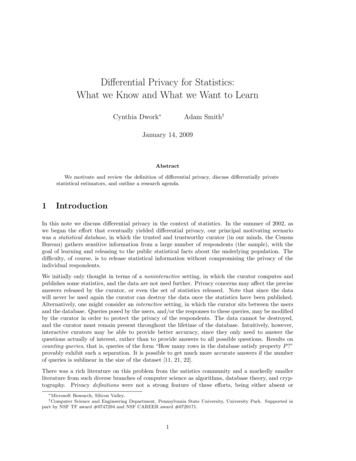
x ) x1 , . . . , x txt 1 , . . . , x2t ?θ̂bc H PPPPPPq. . . xn t 1 , . . . , xn ? ?θ̂bcθ̂bc HH z1 B z2 · · · z k HH j BN average z̄ ?Λnoise R Lap( kε) - - output T z̄ R H Figure 1: The estimator T . When the number of blocks k is ω( n) and o(n2/3 ), and ε is not toosmall, T is asymptotically efficient (Lemma 11).The estimator T takes the data x as well as a parameter ε 0 (which measures information leakage)and a positive integer k (to be determined later). The algorithm breaks the input into k blocks ofn/k points each, computes the (bias-corrected) MLE on each block, and releases the average ofthese estimates plus some small additive perturbation. The procedure is given in Algorithm 1 andillustrated in Figure 1.Algorithm 1 On input x (x1 , ., xn ) Dn , ε 0 and k N:1: Arbitrarily divide the input x into k disjoint sets B1 , ., Bk of t nk points.We call these k sets the blocks of the input.2: for each block Bj {x(j 1)t 1 , ., xjt }, do3:Apply the bias corrected MLE θ̂bc to obtain an estimate zj θ̂bc (x(j 1)t 1 , ., xjt ).4: end forPk15: Compute the average estimate: z̄ kj 1 zj .6: Draw a randomobservationRfromadouble-exponential(Laplace) distribution with standard Λwhere Lap(λ) is the distribution on R withdeviation 2 · Λ/(kε), that is, draw Y Lap kε1 y/λdensity h(y) 2λe . (Recall that Λ is the diameter of the parameter space Θ.) 7: Output T z̄ R.The resulting estimator has the form defT (x) k 1Xθ̂bc x(i 1)t 1 , ., xitk i 1! LapΛkε (4)The following lemmas capture the privacy and utility (respectively) properties of T that implyTheorem 9. Proofs can be found in [54].Lemma 10 ([3, 47]). For any choice of the number of blocks k, the estimator T is ε- differentiallyprivate.1Lemma 11. Under the regularity conditions of Lemma 8, if ε ω( 6 n ) and k is set appropriately,the estimator T is asymptotically unbiased, normal and efficient, that is 1Ln · T (X) N (θ,) if X X1 , ., Xn f (·, θ) are i.i.d.If (θ)8

3.1.3DiscussionAs noted above, Theorem 9 holds for any parametric model where the dimension of the parameterp, is small with respect to n. This covers a number of important settings in classical statistics.One easy example is the set of exponential models (including Gaussian, exponential and loglineardistributions). In fact, a simpler proof of Theorem 9 can be derived for exponential families by addingnoise to their sufficient statistics (using Theorem 6) and computing the MLE based on the perturbedstatistics. Finite mixtures of exponential models (e.g a mixture of 3 Gaussians in the plane) providea more interesting set of examples to which Theorem 9 applies. These are parametric models forwhich no exact sufficient statistics exist short of the entire data set, and so simple perturbativeapproaches seem inappropriate.The technique used to prove Theorem 9 can also be generalized to other settings. For example,it can be applied to any statistical functional which is asymptotically normal and for which biascorrection is possible. Bias correction, in turn, relies only on the bias function itself being smooth.Such functionals include so-called M -estimators quite generally, such as the median or Huber’sψ-estimator.Finally, many of the assumptions can be relaxed significantly. For example, a bounded parameterspace is not necessary, but the “aggregation” function in the construction above, namely the average,must be replaced with a more robust variant. These details are beyond the scope of this paper.3.2Differential Privacy and Robust StatisticsPrivacy-preserving data analysis would appear to be connected to robust statistics, the subfield ofstatistics that attempts to cope with both small errors due, for example, to rounding errors inmeasurements), as well as a few arbitrarily wild errors occuring, say, from data entry failures (seethe books [35] and [34]). In consequence, in a robust analysis the specific data for any one individualshould not greatly affect the outcome of the analysis, as this “data” might in fact be completelyerroneous. This is consonant with the requirements of differential privacy: the data of any oneperson should not significantly affect the probability distribution on outputs. This suggests robuststatistical estimators, or procedures, might form a starting point for designing accurate differentiallyprivate statistical estimators [55]. Dwork and Lei [15] have found this to be the case. They obtained( , ν(n))-differentially private algorithms for the interquartile distance, the median, and regression,with distortion vanishing in n.One difficulty in applying the robust methods is that in robust statistics the assumption is that thereexists an underlying distribution that is “close to” the distribution from which the data are drawn,that is, that the real life distribution is a contamination of a “nice” underlying distribution, andthat mutual dependence is limited. The resulting claims of insensitivity (robustness) are thereforeprobabilistic in nature even when the data are drawn iid from the nicest possible distribution. Onthe other hand, to apply Theorem 6, calibrating noise to sensitivity in order to achieve differentialprivacy even in the worst case, one must cope with worst-case sensitivity.This is not merely a definitional mismatch. Robust estimators are designed to work in the neighborhood of a specific distribution; many such estimators (for example, the median) have high globalsensitivity in the worst case. Dwork and Lei address this mismatch by including explicit, differentially private, tests of the sensitivity of the estimator on the given data set.If the responses indicate high sensitivity, the algorithm outputs “NR” (for “No Reply”), and halts5 .5 Highlocal sensitivity for a given data set may be an indication that the statistic in question is not informative9

Since this decision is made based on the outcome of a differentially private test, no information isleaked by the decision itself – unlike

Di erential privacy is also a very rigid guarantee, since it is independent of the computational power and auxiliary information available to the adversary/user. We can imagine relaxing the assumption that the adversary has unbounded computational power, and we discuss below the extremely useful relaxation to ("; )-di erential privacy.