Transcription
Sample Size Re-estimation in Clinical TrialsChristopher JennisonDepartment of Mathematical Sciences,University of Bath, UKhttp://people.bath.ac.uk/mascjPSI One Day Meeting:Sample size re-estimation — dealing withthose unknownsLondon, 2 November 2016Chris JennisonSample size re-estimation in clinical trials
Outline of talk1. Sample size formulae — what is it that we don’t know?Normal, binary and survival endpoints2. Dealing with nuisance parametersNormal: The variance,Binary:Probability of success on the control arm,Survival: Overall hazard rate3. The unknown treatment effectIs there a problem?Group sequential or adaptive designs?4. ConclusionsChris JennisonSample size re-estimation in clinical trials
1. Sample size formulae(i) A two treatment comparison with normal responseConsider a Phase 3 trial comparing a new treatment with acontrol, where the primary endpoint follows a normal distribution.Denote responses byYBi , i 1, 2, . . . , on the new treatment,YAi , i 1, 2, . . . , on the control arm.A common variance σ 2 is assumed for both treatment and control,so we haveYAi N (µA , σ 2 ) and YBi N (µB , σ 2 ).The treatment effect isθ µ B µA .Chris JennisonSample size re-estimation in clinical trials
A two treatment comparison with normal responseWe wish to test H0 : θ 0 against the alternative θ 0.We set the (one-sided) type I error rate to be α 0.025.We specify an effect size δ we wish to detect with high probability.In order to achieve power 1 β when θ δ, we need a sample sizeof approximately2 (zα zβ )2 σ 2(1)n δ2in both the treatment and control groups. (A more precise answeruses a t-distribution instead of the standard normal distribution.)The sample size formula (1) depends crucially on σ 2 and δ.Practical considerations will favour choices of σ 2 and δ that leadto an affordable trial with a feasible target sample size.Chris JennisonSample size re-estimation in clinical trials
(ii) A two treatment comparison with binary responseConsider a trial with a binary outcome, e.g., success or failure ofthe treatment.Denote responses byYBi , i 1, 2, . . . , on the new treatment,YAi , i 1, 2, . . . , on the control arm,and success probabilities by pA and pB , soYBi 1 with probability pB ,YAi 1 with probability pA .The treatment effect isθ pB pAand we wish to test H0 : θ 0 against θ 0.Chris JennisonSample size re-estimation in clinical trials
A two treatment comparison with binary responseThe success probabilities of treatments A and B are pA and pB .With θ pB pA , we wish to test H0 : θ 0 against θ 0.The (one-sided) type I error rate is α 0.025 and we aim toachieve power 1 β at a specified effect size θ δ.To achieve this power, we need a sample size in each treatmentgroup ofn 2 (zα zβ )2 p̃ (1 p̃),δ2where p̃ (pA pB )/2.Thus, the sample size depends on the specified treatmenteffect δ and the “nuisance parameter” p̃ (pA pB )/2.Chris JennisonSample size re-estimation in clinical trials(2)
(iii) Two treatment comparison with a survival outcomeConsider a Phase 3 trial comparing a new treatment with acontrol, where the primary endpoint is overall survival.Survival times are assumed to follow a proportional hazards modelwith hazard rateshA (t)on the control arm,hB (t) λhA (t) on the new treatment.Let θ log(λ).If the new treatment is successful, λ 1 and θ 0.Thus, we wish to test H0 : θ 0 against θ 0.Chris JennisonSample size re-estimation in clinical trials
A two treatment comparison with a survival outcomeWe test H0 : θ 0 against θ 0 with one-sided type I error rateα 0.025 and we want a high probability of detecting an effectsize θ δ, i.e., a hazard ratio λ eδ , where δ 0.The distribution of the logrank statistic depends on the number ofobserved events (deaths in this case).If the total number of events is n, the unstandardised logrankstatistic is distributed, approximately, asN (θ n/4, n/4).To achieve power 1 β when θ δ, we need a sample size andfollow-up time that will yield a total ofn 2 (zα zβ )2 4δ2events in the treatment and control groups together.Chris JennisonSample size re-estimation in clinical trials(3)
2. Dealing with unknowns in the sample size formulaThe sample size formula, n 2 (zα zβ )2 σ 2 /δ 2 , for the normalcase contains the response variance, σ 2 .Formula (2) for the binary case contains the average success rate p̃.We call σ 2 and p̃ “nuisance parameters”.For survival data, the required number of events in (3) depends on:accrual rate, follow-up, baseline hazard rate and censoring.The internal pilot study approach: Wittes & Brittain (Statist.in Med., 1990) proposed a strategy to achieve desired power.Let φ denote a nuisance parameter in the sample size formula.Design the trial using an initial estimate, φ0 .At an interim analysis, estimate φ from the current data andre-calculate the sample size using this new estimate.Chris JennisonSample size re-estimation in clinical trials
Example: Sample size re-estimation for a varianceA trial is to compare two cholesterol reducing drugs, A and B.The primary endpoint is the fall in serum cholesterol over 4 weeks.The one-sided type I error rate is set at α 0.025 and a power of1 β 0.9 is desired to detect an improvement of 0.4 mmol/L inTreatment B vs Treatment A.Assuming the fall in cholesterol is normally distributed, if theresponse variance is σ 2 , power 0.9 to detect an effect size δ 0.4is achieved by a sample size per treatment ofn 2 (z0.025 z0.1 )2 σ 2.0.42The initial estimate σ02 0.5 gives a sample size per treatment ofn0 2 (1.960 1.281)2 0.5 65.7 66.0.42Chris JennisonSample size re-estimation in clinical trials
Example: Sample size re-estimation for a varianceFollowing the Wittes & Brittain approach, an interim analysis isconducted after observing 33 patients per treatment.Suppose this yields an estimated variance σ̂12 0.62.We re-calculate the sample size per treatment asn1 2 (1.960 1.281)2 0.62 81.4 820.42and increase the total sample size to 82 per treatment arm.We analyse the final data as if from a fixed sample size study.Questions:Does this procedure achieve the overall power of 0.9 when thetreatment effect is 0.4?Is the type I error rate controlled at 0.025?Chris JennisonSample size re-estimation in clinical trials
Example: Sample size re-estimation for a varianceIn our example, suppose the sample size rule is to calculaten1 2 (1.960 1.281)2 σ̂120.42and take the maximum of n1 and 66 as the new sample size pertreatment arm.If the true variance is σ 2 0.6 and this rule is applied,The overall power is 0.899,The type I error probability is 0.0256.This small inflation of the type I error rate is quite typical — thetype I error rate can be as high as 0.03 or 0.04 when the interimanalysis has fewer observations.Chris JennisonSample size re-estimation in clinical trials
Example: Sample size re-estimation for a varianceEven with 64 degrees of freedom to estimate σ 2 at the interimanalysis, the estimate σ̂ 2 is very variable — and, hence, so is thetotal sample size n1 .However, over-estimates compensate for under-estimates inachieving the desired power.Histogram of σ̂ 200.000.0110.0220.030.0430.05Histogram of n10.20.40.60.81.01.2 2σ6080100120140160180200n1Similar variability in total sample size and similar type I error rateinflation are seen for the case of binary response.Chris JennisonSample size re-estimation in clinical trials
Further comments on sample size re-estimation for σ 2Information monitoring and group sequential tests:This method of sample size re-estimation aims for a final estimateof the treatment effect θ with a certain variance.Since “Information” is the reciprocal of Var(θ̂), we are aiming for atarget information level.The same method can be applied in a group sequential test (GST).Mehta & Tsiatis (Drug Information Journal, 2001) implement anerror spending GST where type I error probability is spent as afunction of observed information.A target information level is specified and, unless early stoppingoccurs, the trial continues until this target is reached — withadditional recruitment to increase information if necessary.Chris JennisonSample size re-estimation in clinical trials
Further comments on sample size re-estimation for σ 2Blinded sample size re-estimation:A number of papers address the question of re-estimating samplesize when the treatment labels for each observation are notrevealed (in the interests of maintaining complete blinding).One can fit a mixture of two normal distributions to the pooleddata: see papers by Gould & Shih, Friede & Kieser.Alternatively, one can estimate σ 2 directly from the pooled data —even though this estimate will include a contribution from thedifference in means of the two treatments.Friede & Miller (Applied Statistics, 2012) observe that sample sizemodification based on this form of blinded estimate of σ 2 produceslittle or no type I error rate inflation.Chris JennisonSample size re-estimation in clinical trials
Using a combination test with sample size re-estimationA combination test:Reference: Bauer & Köhne (Biometrics, 1994)Define the null hypothesis H0 (with a one-sided alternative).We shall test H0 : θ 0 vs θ 0, with type I error probability α.Design Stage 1, fixing sample size and test statistic for this stage.Stage 1Observe the P-value P1 for testing H0 .After seeing Stage 1 data, design Stage 2 and fix the test statistic.Stage 2Observe the P-value P2 for testing H0 .Chris JennisonSample size re-estimation in clinical trials
A combination testSuppose θ 0:Then, P1 has the usual U (0, 1) distribution.Also, P2 U (0, 1) conditionally on the Stage 1 data and theresulting Stage 2 design.Since the conditional distribution of P2 is the same for all Stage 1data, P2 is independent of the Stage 1 data (including P1 ).Thus, when θ 0, P1 and P2 are independent U (0, 1) variables.Bauer and Köhne proposed a test based on P1 P2 , using the factthat P1 P2 exp( χ24 /2) when P1 and P2 U (0, 1).Alternatively, one can define a test in terms of the Z-statisticsZ1 Φ 1 (1 P1 ) and Z2 Φ 1 (1 P2 ),which have independent N (0, 1) distributions under θ 0.Chris JennisonSample size re-estimation in clinical trials
The “inverse normal” combination testTo use the inverse normal” combination test, we stipulate that thistest will be used and specify weights w1 and w2 , wherew12 w22 1.The trial is conducted in two stages, with the design of Stage 2 setafter seeing Stage 1 data, as described above.The stage-wise P -values P1 and P2 are calculated, and from thesewe obtain Z1 Φ 1 (1 P1 ) and Z2 Φ 1 (1 P2 ).The overall combination test rejects H0 ifw1 Z 1 w2 Z 2 z α .Since Z1 and Z2 are independent N (0, 1) variables under θ 0,w1 Z1 w2 Z2 N (0, 1)and, hence, the combination test has type I error probability α.Chris JennisonSample size re-estimation in clinical trials
Comments on the inverse normal combination testThe inverse normal combination test rejects H0 ifw1 Z 1 w2 Z 2 z α ,where w1 and w2 are pre-specified weights satisfying w12 w22 1.It may be tempting to adjust the weights w1 and w2 to reflect thesample sizes actually seen in Stages 1 and 2.However, this would undermine the mechanism by which the type Iis protected — and type I error inflation may ensue.Combination tests provide a method to control type I errorprobability precisely in adaptive trial designs.Together, combination tests and multiple testing proceduresunderpin a wide variety of adaptive designs, including seamlessPhase 2/3 designs and enrichment trials.Chris JennisonSample size re-estimation in clinical trials
Example: Sample size re-estimation for a varianceIn the setting of our previous example, we proceed as follows.First stipulate that an inverse normal combination test will be usedwith weights w1 w2 1/ 2.Stage 1Take n0 33 observations per treatment arm,Calculate the t-statisticθb1t1 q2σb21 / 33and find the corresponding P -value P1 P {T64 t1 }.Compute n1 2 (zα zβ )2 σb21 / δ 2 and set the Stage 2 samplesize per treatment to be n2 max(n1 , 66) 33.Chris JennisonSample size re-estimation in clinical trials
Example: Sample size re-estimation for a varianceStage 2Take n2 observations per treatment arm,Calculate the t-statistic based solely on Stage 2 dataθb2t2 q2σb22 / n2and find the P -value P2 P {T2n2 2 t2 }.The overall combination testFind Z1 Φ 1 (1 P1 ) and Z2 Φ 1 (1 P2 ).Using the pre-specified weights, reject H0 : θ 0 if (1/ 2) Z1 (1/ 2) Z2 zα .Chris JennisonSample size re-estimation in clinical trials
Properties of the trial design using a combination testIn the above design, we take an initial sample of n0 33 pertreatment, then calculaten1 2 (1.960 1.281)2 σ̂12 /0.42 ,and take a further {max(n1 , 66) 33} patients per treatment arm.If the true variance is σ 2 0.6 the Wittes & Brittain method gaveType I error probability 0.0256,Overall power 0.899Using the inverse normal combination test, we haveType I error probability 0.0250,Overall power 0.896.Chris JennisonSample size re-estimation in clinical trials
Sample size re-estimation with a binary responseExample: Treatment for heart failureA new treatment is to be compared to the current standard.The primary endpoint isRe-admission to hospital (or death) within 30 days.The current treatment has a re-admission rate of 25%.Testing for superiorityIt is hoped the new treatment will reduce re-admissions to 20%.Denote re-admission probabilities by pt on the new treatment andpc on the control.To establish superiority of the new treatment, we test H0 : pt pcagainst pt pc — hoping to reject H0 .Chris JennisonSample size re-estimation in clinical trials
Binary example: Treatment for heart failureSetting θ pc pt , we wish to test H0 : θ 0 against θ 0 withType I error rate: α 0.025 at θ 0,Power: 1 β 0.9 when θ δ 0.25 0.2 0.05.From (2), we achieve this power with a sample size of2 (zα zβ )2 p̃ (1 p̃),δ2in each treatment group, where p̃ (pc pt )/2.n From historical data, we expect pc 0.25.With pt 0.2, this gives p̃ (0.25 0.2)/2 0.225, and therequired sample size test per treatment arm isn0 1466.Chris JennisonSample size re-estimation in clinical trials
Binary example: Treatment for heart failureThe sample size formula depends on pc , as well as θ pc pt .Desired power may not be achieved if previous data are notrepresentative of the new study: for example, hospitals involvedmay have a different case mix and admit more seriously ill patients.Suppose investigators decide to conduct an interim analysis atwhich an increase in sample size may be agreed.The trial designA Bauer & Köhne two-stage design is specified.Data from before and after the interim analysis will be combined using an inverse normal combination test with w1 w2 1/ 2.The initial calculation gave a target sample size of n0 1466 pertreatment arm: we recruit 730 patients per treatment in Stage 1.Chris JennisonSample size re-estimation in clinical trials
Binary example: Treatment for heart failureStage 1, with 730 subjects per treatment, yields p̂c 0.253 andp̂t 0.219, so θb 0.034 with standard error 0.0222.A test of H0 : θ 0 has Z1 0.034/0.0222 1.531.The overall test will reject H0 if (1/ 2) Z1 (1/ 2) Z2 zα 1.96. Since Z1 / 2 1.083, results thus far are promising. However, apositive outcome is by no means certain.Investigators learn that trials of competing treatments have beenunsuccessful.It is decided to increase the second stage sample size to give higherprobability of a positive outcome under the original alternative,θ 0.05 — and under smaller effect sizes.Chris JennisonSample size re-estimation in clinical trials
Binary example: Planning the Stage 2 sample sizeImplications of several sample size choices are summarised below.pcptθStage 2sample 05750100012500.860.920.96Investigators increase Stage 2 sample size to 1000 per treatment.Chris JennisonSample size re-estimation in clinical trials
Binary example: Treatment for heart failureWith 1000 subjects per treatment, Stage 2 data (alone) yieldp̂c 0.248 and p̂t 0.223.Thus, θb 0.025 with standard error 0.0190.A test of H0 : θ 0 based on Stage 2 data has Z-statistic0.025/0.0190 1.318.In the overall test, Z1 / 2 Z2 / 2 (1.531 1.318)/ 2 2.013 zα .Thus, the null hypothesis H0 : θ 0 is rejected and the newtreatment is recommended for use.We have dealt with unknown “nuisance parameters” — andwe have seen other reasons for a change in sample size.Chris JennisonSample size re-estimation in clinical trials
3. The unknown treatment effectIn the last example, we saw the opportunity to increase sample sizein order to increase power under smaller treatment effects.It seems quite reasonable to do this in response to externalinformation that was not available when the trial was designed.b of theShould one do this in response to an interim estimate, θ,treatment effect?In the sample size formulaen 2 (zα zβ )2 σ 2δ2(normal case),n 2 (zα zβ )2 p̃ (1 p̃)δ2(binary case),is δ an “unknown”?Chris JennisonSample size re-estimation in clinical trials
Choosing the effect size δ for the sample size formulaWe denote by θ the effect size of a new treatment, i.e., thedifference in mean response between the new treatment and thecontrol.If we wish the trial to have power 1 β when θ δ, we put theeffect size δ in the sample size formula.Dispute can arise over the choice of δ.For example, should investigators use:The minimum effect of interest 1 , orThe anticipated effect size 2 ?Chris JennisonSample size re-estimation in clinical trials
An example: Specifying the effect size δ1.0Suppose sample sizes of 500 and 1000 give these power curves:0.20.4Power0.60.8n 1000n 5000.0 0.00.51.011.5 22.02.53.0θWith 1000 subjects, there is good power at the minimum clinicallysignificant effect, 1 .With only 500 subjects, a high power is achieved at the moreoptimistic 2 — but there is not a lot of power at 1 .If θ 2 , a sample size of 1000 is unnecessarily high.Chris JennisonSample size re-estimation in clinical trials
An example: Specifying the effect size δA sample size of 500 would be sufficient if θ 2 .However, if θ 1 we would like to have the power provided by asample size of around 1000.An adaptive strategy: Start small then ask for moreStart with a planned sample size of 500,Look at the results of the first 250 observations,If appropriate, increase the sample size to 1000.The group sequential approachStart with a maximum sample size of 1000,Conduct one or more interim analyses,Stop early if there is enough evidence to do so.Chris JennisonSample size re-estimation in clinical trials
Comparing different types of trial designAll designs have overall power and Eθ (N ) curves.Eθ (N ) 5001.0Power curve 101234θ 101234θDesigns with similar power curves can be compared in terms oftheir average sample size functions, Eθ (N ).Even if investigators are uncertain about the likely treatmenteffect, they can usually specify values of θ under which earlystopping is most desirable.Chris JennisonSample size re-estimation in clinical trials
Adaptive or group sequential designs?Jennison & Turnbull have studied optimal versions of adaptive andnon-adaptive sequential designs (e.g., Statist. in Med., 2003 and2006, Biometrika, 2006). They report:The set of group sequential tests(GSTs) is a subset of the set ofadaptive designs,And advice is available onhow to create good groupsequential designs:Adaptive designs are, at best, alittle more efficient than GSTswith the same number of analyses,reducing average sample size by1% or 2% for the same power,Many published adaptive designsare considerably less efficient thana well chosen GST.Chris JennisonSample size re-estimation in clinical trials
What to look for in a trial designIf you are considering a trial design with sample size re-estimationin response to an interim estimate of the treatment effect, then:Look at the power function and Eθ (N ) curve,Compare with Eθ (N ) for a standard GST, e.g., from theρ-family of error spending tests (J & T, Ch. 7).You should be wary of a sample size rule that treats an interim θbas an accurate estimate of the true θ:In the Heart Failure example, we wanted power 0.9 todifferentiate between θ 0 and θ 0.05,The interim estimate θb 0.034 had a standard error of0.0222, giving a 95% CI for θ of ( 0.01, 0.08),This scale of standard error of θb is typical.Chris JennisonSample size re-estimation in clinical trials
Some comments on the “Promising Zone” approachMehta & Pocock (Statist. in Med., 2010) proposed a particularform of sample size re-estimation in their paper:“Adaptive increase in sample size when interim resultsare promising: A practical guide with examples”In their Example 1, response is measured 26 weeks after treatment,causing problems for standard group sequential tests.At the interim analysis, there is a large number of “pipeline”patients who have been treated but are yet to produce a response.Jennison & Turnbull focus on this example in their (Statist. inMed., 2015) paper“Adaptive sample size modification in clinical trials:start small then ask for more?”Chris JennisonSample size re-estimation in clinical trials
Properties of the Mehta-Pocock design0.4Power0.60.81.0M & P use a result of Chen, DeMets & Lan (Statist. in Med.,2004) that allows an increase in sample size (in certain situations)to be followed by a standard, fixed sample size analysis at the endof the trial.0.2MP adaptive design0.0Fixed N 442 101234θJ & T note that the limited opportunity for increasing sample sizeleads to only a small increase in overall power.Chris JennisonSample size re-estimation in clinical trials
Alternatives to the MP design for their Example 11200J & T explore other ways of achieving the power of MP’s design.MP adaptive designFixed N 490n 202004006008001000GSD R 1.05 101234θ 11. A fixed sample size design with 490 observations (cf, theminimum of 442 for MP)2. A group sequential test that stops after with a sample size of416 or 514. If the GST stops at the first analysis, responses fromthe 208 pipeline subjects are not used — but these patients arecounted in Eθ (N ).Chris JennisonSample size re-estimation in clinical trials
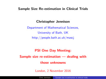
Alternatives to the MP design for their Example 1Eθ (N ) curves480460MP adaptive designMP adaptive designFixed N 490Fixed N 490GSD R 1.054000.2420440Eθ(N)0.60.4Power0.85001.0Power curve3800.0GSD R 1.05 101234θ 101234θAll three designs have essentially the same power curve.The fixed sample design has lower Eθ (N ) than the MP design overthe θ values of most interest.The GST has uniformly lower Eθ (N ) than the MP design.Chris JennisonSample size re-estimation in clinical trials
Alternatives to the MP design for their Example 1J & T go on to develop a method in the adaptive framework(“start small and ask for more”) that lowers the Eθ (N ) curvewhile maintaining power.Eθ (N ) curves5001200Sample size rulesMP adaptive design480460MP adaptive design400200420440Eθ(N)600400n 28001000CT Min E(N) at θ 1.6, min n 2 416Density of θ 1 (θ 1.6)0380CT Min E(N) at θ 1.6, min n 2 416 101234 10θ 11234θJ & T use an inverse normal combination test.They also employ a “rate of exchange” between sample size andpower to ensure a consistent approach to the choice of sample size.Chris JennisonSample size re-estimation in clinical trials
4. ConclusionsSample size re-estimation in response to information aboutnuisance parameters can help in achieving a desired power curve.In doing this, the use of combination tests avoids any inflation ofthe type I error rate.Group sequential tests provide a mechanism for responding toinformation about the treatment effect — by stopping the trialat an interim analysis.GSTs are tried and tested, and special forms of GST have beendeveloped to deal with unequal group sizes and delayed response(see Hampson & Jennison, J. Roy. Statist. Soc., B, 2013).Some adaptive designs match the performance of good GSTs.However, some other adaptive designs do not.Chris JennisonSample size re-estimation in clinical trials
achieve power 1 at a speci ed e ect size . To achieve this power, we need a sample size in each treatment group of n 2(z z )2 p (1 p ) 2; (2) where p (p A p B) 2. Thus, the sample size depends on the speci ed treatment e ect and the \nuisance parameter" p (p A p B) 2. Chris Jennison Sample size re-estimation in clinical trials