Transcription
Downloaded from orbit.dtu.dk on: Aug 11, 2022CFD code comparison for 2D airfoil flowsSørensen, Niels N.; Mendez, B.; Munoz, A.; Sieros, G.; Jost, E.; Lutz, T.; Papadakis, G.; Voutsinas, S.;Barakos, G. N.; Colonia, S.Total number of authors:13Published in:Journal of Physics: Conference Series (Online)Link to article, DOI:10.1088/1742-6596/753/8/082019Publication date:2016Link back to DTU OrbitCitation (APA):Sørensen, N. N., Mendez, B., Munoz, A., Sieros, G., Jost, E., Lutz, T., Papadakis, G., Voutsinas, S., Barakos, G.N., Colonia, S., Baldacchino, D., Baptista, C., & Ferreira, C. M. D. (2016). CFD code comparison for 2D airfoilflows. Journal of Physics: Conference Series (Online), 753, [082019]. al rightsCopyright and moral rights for the publications made accessible in the public portal are retained by the authors and/or other copyrightowners and it is a condition of accessing publications that users recognise and abide by the legal requirements associated with these rights. Users may download and print one copy of any publication from the public portal for the purpose of private study or research. You may not further distribute the material or use it for any profit-making activity or commercial gain You may freely distribute the URL identifying the publication in the public portalIf you believe that this document breaches copyright please contact us providing details, and we will remove access to the work immediatelyand investigate your claim.
HomeSearchCollectionsJournalsAboutContact usMy IOPscienceCFD code comparison for 2D airfoil flowsThis content has been downloaded from IOPscience. Please scroll down to see the full text.2016 J. Phys.: Conf. Ser. 753 82019)View the table of contents for this issue, or go to the journal homepage for moreDownload details:IP Address: 130.226.56.2This content was downloaded on 27/10/2016 at 14:14Please note that terms and conditions apply.You may also be interested in:Numerical simulations of the NREL S826 airfoilKF Sagmo, J Bartl and L SætranLES tests on airfoil trailing edge serrationWei Jun Zhu and Wen Zhong ShenSimulation and Optimization of an Airfoil with Leading Edge SlatMatthias Schramm, Bernhard Stoevesandt and Joachim PeinkeExperimental benchmark and code validation for airfoils equipped with passive vortex generatorsD Baldacchino, M Manolesos, C Ferreira et al.Numerical and experimental investigation of an airfoil with load control in the wake of an activegridA Fischer, T Lutz, E Kramer et al.Aero-Acoustic Modelling using Large Eddy SimulationW Z Shen and J N SørensenDynamic lift measurements on a FX79W151A airfoil via pressure distribution on the wind tunnel wallsGerrit Wolken-Möhlmann, Pascal Knebel, Stephan Barth et al.
The Science of Making Torque from Wind (TORQUE 2016)Journal of Physics: Conference Series 753 (2016) 082019IOP Publishingdoi:10.1088/1742-6596/753/8/082019CFD code comparison for 2D airfoil flowsNiels N. Sørensen1 , B. Méndez2 ,A. Muñoz2 , G. Sieros3 , E. Jost4 ,T.Lutz4 , G. Papadakis5 , S. Voutsinas5 , G.N. Barakos6 , S. Colonia6 , D.Baldacchino7 ,C. Baptista7 , C. Ferreira71234567DTU Wind Energy, Technical University of Denmark, Risø Campus, Denmark.CENER, Av Ciudad de la Innovacion 7, Sarriguren 31621, Navarra, SpainCRES, Wind Energy Dept., Pikermi, GreeceInstitute of Aerodynamics and Gas Dynamics, University of Stuttgart, GermanyNational Technical University of Athens, GreeceSchool of Engineering, University of Glasgow, U.K.Delft University of Technology, The NetherlandsE-mail: nsqr@dtu.dkAbstract. The current paper presents the effort, in the EU AVATAR project, to establish thenecessary requirements to obtain consistent lift over drag ratios among seven CFD codes. Theflow around a 2D airfoil case is studied, for both transitional and fully turbulent conditions atReynolds numbers of 3 106 and 15 106 . The necessary grid resolution, domain size, anditerative convergence criteria to have consistent results are discussed, and suggestions are givenfor best practice. For the fully turbulent results four out of seven codes provide consistentresults. For the laminar-turbulent transitional results only three out of seven provided results,and the agreement is generally lower than for the fully turbulent case.1. IntroductionIn connection with the EU AVATAR project, dealing with the aerodynamics and aeroelasticityof the wind turbines of the future, a large effort is invested in the exploration of ComputationalFluid Dynamics (CFD) codes. The continuous upscaling of wind turbines requires codevalidation for new flow regimes, where the Reynolds numbers increase above 10 106 , andthe Mach numbers may be in the range [0.01:0.3]. In this region, experimental data relevantto wind turbines are sparse and costly to obtain. In the EU AVATAR Project a three stepprocedure is used to solve this problem: Establish the necessary requirements for several CFD solvers to provide consistent results. Validate the CFD solvers on the sparse data available. Apply the solvers to explore the target flow regime.Finally, the results from the CFD solvers will be used to develop the engineering methods usedin industry to handle the upscaled turbines.The present work deals with a code comparison, that aims at establishing the requirementfor the solvers to consistently predict both fully turbulent and transitional 2D airfoil flows. Thefocus is on conditions where the Mach number is 0.1 while the Reynolds number is varied froma moderate value of 3 106 to a high value of 15 106 . The conditions corresponds to a recentContent from this work may be used under the terms of the Creative Commons Attribution 3.0 licence. Any further distributionof this work must maintain attribution to the author(s) and the title of the work, journal citation and DOI.Published under licence by IOP Publishing Ltd1
The Science of Making Torque from Wind (TORQUE 2016)Journal of Physics: Conference Series 753 (2016) 082019IOP Publishingdoi:10.1088/1742-6596/753/8/082019wind tunnel test of the DU00-W-212 airfoil, performed in the AVATAR project. Several ofthe codes have a long track record, and have previously been validated against data in severalstudies, both in connection with blind comparisons, and against data from the open literature,[29, 30, 28, 10, 23, 2].The main focus is to investigate the requirement of the codes to have consistent solutionsfor the target flow regimes, in terms of the necessary domain size, grid resolution, and iterativeconvergence criteria. Even though the issue of obtaining iterative and grid convergence ofnumerical methods is not new, it is still an essential problem, see [24, 25, 5].2. MethodsBoth compressible and incompressible Reynolds Averaged Navier-Stokes (RANS) methods areapplied. All solvers apply the k ω SST turbulence model by Menter [12], while different typesof transition models are applied. The computations are carried out in time or iteration, until thevariation over the last 10 percent of the integration time or iterations, are within 0.05 percentfor the lift, and 0.1 percent for the drag. For most of the solvers, the L2 norm of the residualsare reduced by 5-6 orders of magnitude to assure this.The CENER calculations are performed using the code WMB [6]. The code is a structuredmulti-block cell-centred finite volume method, based on the compressible Unsteady ReynoldsAveraged Navier-Stokes (URANS) equations. The calculations are done in steady state usingthe k ω SST turbulence model for the fully turbulent calculations, and k ω SST combinedwith the eN method for the transitional ones.The CRES computations are performed using an incompressible implicit pressure correctionsolver. The algorithm introduces a matrix-free algorithm for pressure updating, whichmaintains the compatibility of the velocity and pressure field corrections, allowing for practicallyunlimited large time steps in steady state calculations. Spatial discretisation is performed ona computational domain, resulting from a body fitted coordinate transformation using finitevolume schemes. The velocity is stored at grid nodes, while the pressure is computed at midcells. A linear 4th order pressure dissipation term is added into the continuity equation toprevent velocity-pressure decoupling. Further details can be found in [3]. For turbulent flowcomputation, the standard k ω or the k ω SST [13] models can be used. In the present paperall results are produced with the k ω SST for fully turbulent flow.The DTU computations are performed in steady state using the EllipSys2D in-houseincompressible finite volume RANS flow solver, see [18, 19], [26]. The convective terms arediscretised using the QUICK scheme, as given by [9]. The turbulent simulations are carried outusing Menter’s k ω SST model described in [12], while the transitional simulations are basedon the eN transition model, as described in [20].The NTUA computations are performed using the MaPFlow in-house compressible finitevolume RANS flow solver. The implementation uses Roes scheme, low Mach preconditioning,and non-preconditioned far-field conditions in Riemann invariant form [22]. Menters k ω SSTturbulence closure model [12], and the eN transition model as described in [4] are used. In thepresent simulations limiters are suppressed. For angles of attack outside of the range [-11:11],unsteady simulations are performed.The TUDelft calculations are performed using OpenFOAM v2.3.0, an open source CFDsoftware distributed under the General Public Licence (GPL), see[7]. OpenFoam is a segregatedfinite volume code able to solve compressible and incompressible flows. For this work, thesteady, incompressible RANS equations are solved using the SIMPLE algorithm. The governingequations are solved using first order upwind discretisation schemes for the convective terms.Fully turbulent simulations use Menter’s two-equation k-ω SST model [12]. Transitionalsimulations are conducted using the kkl-ω model [35], which solves for the laminar and turbulentkinetic energy, as well as a third transport equation which governs low-frequency velocity2
The Science of Making Torque from Wind (TORQUE 2016)Journal of Physics: Conference Series 753 (2016) 082019Topo.OC-HC-HChord-wiseNr. CellsAirfoil/Wake384/401/125422/155NormalNr. Cells192155156TE BlockNr. CellsWake x TE125 61155 75 n[Chords]1 10 61 10 61 10 6IOP Publishingdoi:10.1088/1742-6596/753/8/082019Domain Size[Chords]Normal/Wake40/4040/4025/25Nr. ble 1. Mesh topologies used in the simulations.fluctuations that trigger transition in the boundary layer.The UOG computations use the Helicopter Multi-Block (HMB3) code [2], a cell-centredRANS finite volume approach. The solver uses a fully-implicit time integration. Followingthe pseudo-time approach, after the linearisation of the residual at the new pseudo time step,the discretised RANS result in a large system of linear equations. In HMB3, the latter issolved employing a Generalised Conjugate Gradient (GCG) method [1], pre-conditioned with anIncomplete Lower Upper (ILU) factorisation[11]. To discretise the convective part of the NavierStokes equations, a formally third order Monotone Upstream-Centred Scheme for ConservationLaws (MUSCL) [33] is employed with the Van Albada limiter [34]. In the present work, the Osherscheme [21] is used for the fluxes, and the turbulent closure is the k ω SST model of Menter[13]. When the laminar-turbulent transition is considered, the k ω SST turbulence modelis coupled with the γ equation LCTM of Menter [17]. A second order central discretisationscheme is used for the viscous fluxes.The USTUTT simulations are performed with the CFD code FLOWer, which is developedby the German Aerospace Center (DLR), see [8]. FLOWer is a compressible code that solvesthe RANS equations in integral form. The numerical scheme is based on a finite-volumeformulation for block-structured grids. To determine the convective fluxes, a second ordercentral discretisation with artificial damping is used, also called the Jameson-Schmidt-Turkel(JST) method. Time integration is accomplished by an explicit multi-stage scheme includinglocal time-stepping. The time-accurate simulations make use of the implicit Dual-time-steppingmethod. In the present study, the simulations are performed in steady and unsteady mode ifneeded for converged loads. Turbulence modelling is accomplished by the Menter’s k ω SSTmodel described in [12].2.1. Grid GenerationA common grid is provided for all partners to serve as a reference point, generated by thehyperbolic grid generation code HypGrid2D [27] around the DU00-W-212 airfoil [32]. The gridhas a single block O-topology with a finite sharp trailing edge, and a total of 73728 cells. Thegrid has 384 cells in the chord-wise direction and 192 cells in the normal direction, placing theouter boundary 40 chords away from the airfoil. The cell spacing in normal direction has a y/Chord 1.5 10 6 , which should assure that y is below 2 for both the considered Reynoldsnumbers. At the finite trailing edge 16 cells are distributed with a cell size of s/Chord 2 10 4at the sharp corners. At the leading edge the cell size is set to s/Chord 1 10 3 . Thestretching in the chord-wise and normal directions is accomplished by double sided tanhstretching functions, giving low expansion rates. Most partners are using the common grid, buttwo partners used their own grids, namely the UOG and CENER. Additionally, some partnerstested other mesh topologies (C, OCH), resolutions, and domain sizes.Even though CENER tested the common O-mesh, the results presented here is computed ona C-H meshes topology generated in ANSYS ICEMCFD, and coarsened by the same method asthe common grid, see Table 1. The UOG computations are performed on a special C-H mesh,3
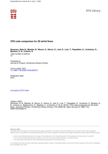
The Science of Making Torque from Wind (TORQUE 2016)Journal of Physics: Conference Series 753 (2016) 082019IOP Publishingdoi:10.1088/1742-6596/753/8/082019Figure 1. Details of the grids near the surface for the described grid coarsening from left toright, L1, L2, and L3.where the coarser grids are regenerated reducing the number of points by a factor of 2.5 (L2)and 3.5 (L3) keeping the y constant.2.2. Grid refinement methodAs the applied common grid is a block structured grid, the grid refinement/coarsening approachis kept simple. The coarser grid is constructed from the finest grid (L1) by removing everysecond point in both directions, resulting in the medium grid (L2). By repeating the coarseningprocedure even coarser levels can be obtained. Here the coarsening is limited to two consecutivetimes, resulting in three grid levels, the finest L1, the medium L2, and the coarsest L3, seeFigure 1The advantage of this approach, identical to the approach which has been used within theEllipSys solver for years to do grid-sequencing, is that it is a very tough test where all parametersare varied at the same time. The cell size, the y value at the wall surface, and the grid expansionrate is more than doubled, while the number of cells within the boundary layer is halved. Lookingat the glide ratio, focusing on the AOA region between [-5:9] degrees the discretisation error forthe best performing code is around 2 percent. The discretisation error of most of the codes are 47 percent. For three of the codes, the discretisation error is more than 10 percent. It is importantto remember that grid independence does not guarantee that the solution is approximating thephysics, only that the solution is a true representation of the implemented models.2.3. Far-field boundary conditionInitial investigations revealed that even with a domain size of 40 Chords, a point vortex correctionis needed by some solvers to account for the induced velocity in the far-field and to provide adomain size independent solution on the common O-mesh, eg. the FLOWer solver. Other solversworked well for the common O-mesh configuration, while CH- and OCH-meshes, constructedwith a similar domain size, revealed the need for a vortex correction on these topologies toavoid influence on the integral quantities from the pressure disturbance in the far-field, eg. theEllipSys2D solver. The influence from a lifting airfoil on its surroundings can be approximatedfrom simple potential flow, using the Kutta-Jukowski theorem and the Biot-Savart law, resultingin the following boundary condition at the outer boundary:Uθ U Clr4π Chord(1)where Cl is the Lift coefficient per unit span, U is the free stream velocity, and r/Chord isthe normalized distance from the domain centre. As an alternative to applying the point vortexcorrection, the expression can be used to determine the necessary domain size to reduce theneglected induced velocity at the far-field below a given threshold value. The effect of including4
The Science of Making Torque from Wind (TORQUE 2016)Journal of Physics: Conference Series 753 (2016) 082019IOP Publishingdoi:10.1088/1742-6596/753/8/082019Figure 2. The effect of a point vortex correction on the pressure, illustrated by iso-bars showingthe uncorrected results on an O- and OCH-mesh left and the corrected results right, based onthe EllipSys2D results. The red colours represents high pressure values, while the blue coloursrepresent low pressure values.the vortex correction in the EllipSys2D computations is illustrated in Figure 2, where it isevident that the correction limits the distortion of the iso-bars near the outer boundary.3. Results3.1. Fully turbulent resultsA direct comparison of all partner results on the finest grid level (L1) with respect to the glideratio (Cl/Cd), is shown in Figure 3. Here all partners are shown with identical colour, with thesole intention of indicating the spread. The glide ratio is an important parameter in connectionwith wind turbine design, and additionally a highly sensitive parameter. At the maximum glideratio, the difference in the glide ratio at the low and high Reynolds numbers are 8 and 18 percent,respectively.In Figure 4, a representative example of the spread between the seven individual results isillustrated. As seen in the left side of the figure, the pressure distributions are in very goodagreement, and only one of the codes can be seen to deviate slightly. For the skin-friction, oneof the codes show some numerical wiggles, while the remaining codes show acceptable mutualagreement.A representative picture can be seen when comparing the grid dependence of the glide ratiocomputed by the different solvers for the fully turbulent simulation at Re 15 106 , usingconsecutive coarsenings of the grids, see Figure 6. Several of the solvers do not provide gridindependence results, even in the attached flow region of [-8:10] degrees, where RANS solvers areexpected to provide good predictions. It is also evident from this figure, that grid dependencevaries with the AOA. Based on this, it is concluded that the grid dependence must be investigatedfor the full AOA range of interest.5
The Science of Making Torque from Wind (TORQUE 2016)Journal of Physics: Conference Series 753 (2016) 08201980IOP -15-10-5051015-100-2020-15-10-5Aoa [deg]05101520Aoa [deg]Figure 3. The spread in the glide ratio predicted by the individual partners, fully turbulentconditions at Re 3 106 left, and Re 15 106 ordFigure 4. A comparison of the predicted pressure, and skin-friction distributions for all partnersat a Reynolds number of 3 106 , and an angle of attack of 4 degrees. The figures are solelyshown to indicate the spread, and all partners are shown with identical -40-60-20-60-15-10-5051015-80-2020Aoa [deg]-15-10-505101520Aoa [deg]Figure 5. Glide ratio predicted by four of the seven codes, fully turbulent conditions atRe 3 106 left, and Re 15 106 right.6
IOP 100100808060604040Cl/CdCl/CdThe Science of Making Torque from Wind (TORQUE 2016)Journal of Physics: Conference Series 753 (2016) 082019202000-20-20-40-80-20-40DTU, L1DTU, L2DTU, L3TUD, L1-60-15-10-50510TUD, L1TUD, L2TUD, L3DTU, -20-20-40-40NTUA, L1NTUA, L2NTUA, L3DTU, 0Aoa [deg]12012010010080806060404020Cl/CdCl/Cd10CRES, L1CRES, L2CRES, L3DTU, L1-60Aoa [deg]0200-20-20-40-40CENER-WMB, L1CENER-WMB, L2CENER-WMB, L3DTU, L1-60-80-100-205200-80-200Aoa [deg]Cl/CdCl/CdAoa [deg]-15-10-50510UOG, L1UOG, L2UOG, L3DTU, L1-6015-80-2020-15-10-5Aoa [deg]0510Aoa [deg]1201008060Cl/Cd40200-20-40USTUTT, L1USTUTT, L2USTUTT, L3DTU, L1-60-80-20-15-10-505101520Aoa [deg]Figure 6. Grid dependency of the fully turbulent results for the individual partners atRe 15 106 .7
The Science of Making Torque from Wind (TORQUE 2016)Journal of Physics: Conference Series 753 (2016) 2570.0115TUD1.22490.0118IOP 19200.0115UOG1.21950.0125CENER1.23160.0110Table 2. Lift and drag at an angle of attack equal to 8 degrees for fully turbulent conditionsat Re 15 106 .As grid independence is a necessary prerequisite for comparing the solution between differentsolvers, the three solvers having the highest variability with grid refinement from level 2 to level1 are excluded, and the four remaining solvers are compared. Comparing the four remainingsolvers, see Figure 5, the deviation between the solvers is down to less than 2 percent in glideratio. Looking at the lift and drag values at 8 degrees, close to maximum glide ratio, it can bederived from Table 2 that most codes are agreeing within 0.25 percent in lift, and 2 percent indrag.3.2. Results including the laminar-turbulent transition processA similar exercise is done for the transitional cases, looking again at Reynolds numbers of 3 106and 15 106 . In the present study, only three codes were applied successfully to the transitionalcomputations, all based on the eN type transition models. Results are not included for thecorrelation based transition model by Menter and Langtry [15], [16], available in some of thecodes, as it fails to correctly predict the natural transition behaviour at high Reynolds numbers.This was first experienced by some of the authors in connection with the studies of the DTU 10MW turbine, in the INNWIND EU project back in 2013, and illustrated in some detail in 2014[31].Looking at the glide ratio, as shown in Figure 7, several tendencies are similar to theobservations for the fully turbulent computations. Two out of the three codes have only minorvariation in glide ratio between the finest grid level L1, and the coarser L2, for angles between[-10:10]. The third code exhibits large differences between the two finest grid levels, similar toits fully turbulent behaviour. Even though the third code exhibits a large variation from L2 toL1, the actual computed values on L1 is close to the values computed by the two other codes.To verify whether the result of the third code on grid L1 is grid independent, a refined versionof the L1 grid was generated and tested. The results are not shown here, but the solution on therefined grid showed good agreement with the L1 solution. Generally, the transitional results areshowing larger spread than the fully turbulent results, which indicate that transition predictionis not as well tested as the fully turbulent approach.4. DiscussionSeveral lessons were re-learned by the partners during the exercise, when going into the newregime of high Re and low Mach that will be experienced on wind turbines in the future.Grid generation has to be done very carefully. This implies using e.g. hyperbolic tangentstretching to limit the expansion rate in the high gradient regions, both chord-wise and in thenormal direction. At the high Reynolds numbers dealt with here, the very small cells needed atthe wall will result in slow iterative convergence for many solves. Comparing the results fromthe seven codes is illustrative, and it is observed that for codes formally of second order, thegrid requirement to obtain grid independent results might differ.The effect of the domain size is illustrated, and it is concluded that a large domain size ofthe order of 100 chords or including a vortex correction, is necessary to have consistent resultsbetween the codes.8
The Science of Making Torque from Wind (TORQUE 2016)Journal of Physics: Conference Series 753 (2016) 082019IOP 5050Cl/Cd150Cl/Cd15000-50-100-20-50DTU, Level-1DTU, Level-2DTU, Level-3NTUA, Level-1-15-10-5051015-100-2020DTU, Level-1DTU, Level-2DTU, Level-3NTUA, Level-1-15-10-5Aoa [deg]0510152015201520Aoa [deg]1001005050Cl/Cd150Cl/Cd15000-50-100-20-50DTU, Level-1NTUA, Level-1NTUA, Level-2NTUA, Level-3-15-10-5051015-100-2020DTU, Level-1NTUA, Level-1NTUA, Level-2NTUA, Level-3-15-10-5Aoa [deg]0510Aoa 0-50DTU, Level-1CENER-WMB, Level-1CENER-WMB, Level-2CENER-WMB, Level-3-40-15-10-5051015-100-2020Aoa [deg]DTU, Level-1CENER-WMB, Level-1CENER-WMB, Level-2CENER-WMB, Level-3-15-10-50510Aoa [deg]Figure 7. Grid dependency of the individual partner results for transitional results, leftRe 3 106 , and right Re 15 106 .Additionally, it was observed that the individual formulations require a very different numberof iteration or time-steps to converge. The fastest solver might require less than 1000 iterations,while others required more than 20000 iterations. The efficiency with respect to computing time,not discussed here, will depend on the cost of the iteration or time-step.For the laminar-turbulent transitional computations, only three partners contributed withresults. Even though the standard correlation based model is available in some of the codes,it is not applied due to the problem of predicting the natural transition on an airfoil at highReynolds numbers. Generally, the three codes predict results in decent agreement, even thoughit is not as good as for the fully turbulent computations. Finally, it was illustrated that griddependency should be investigated at all angles of attack of interest. For structured grids, a9
The Science of Making Torque from Wind (TORQUE 2016)Journal of Physics: Conference Series 753 (2016) 082019IOP Publishingdoi:10.1088/1742-6596/753/8/082019simple coarsening where every second cell is removed in the chord-wise, and the normal direction,is well suited for the purpose.5. ConclusionThis paper presents the effort to make seven different RANS CFD solvers provide consistentresults. Even though the results are not fully satisfactory for all solvers, four out of sevencodes are capable of predicting the maximum glide-ratio with a difference below 2 percent forfully turbulent conditions. To obtain this level of agreement domain size, careful treatment ofboundary conditions, grid quality, and iterative convergence must be in focus.More work is need to fully establish the application of laminar-turbulent transition modelsfor the flow regime of the wind turbines of the future. This conclusion is based on the fact thatseveral codes are not capable of providing transitional results, and that the mutual agreementbetween the results from the codes are inferior to the fully turbulent behaviour.5.1. AcknowledgementsThe present research is funded by the EU AVATAR project No FP7-ENERGY-2013-1/no.608396, Advanced Aerodynamic Tools for Large Rotors.6. References[1] O. Axelsson. Conjugate Gradient Type Methods for Unsymmetric and inconsistent System of LinearEquation. Linear Algebra and its Applications, 29:1–16, 1980.[2] G. Barakos, R. Steijl, A. Brocklehurst, and K. Badcock. Development of CFD Capability for Full HelicopterEngineering Analysis. In 31st European Rotorcraft Forum, pages 19–29, 2005.[3] P. Chaviaropoulos. A Matrix-Free Pressure Solver for the Incompressible Navier-Stokes Equations Application to 2-D Flow. Proceedings of ECCOMAS Conference, Stuttgart, Germany, 1994[4] M. Drela and M. B. G. . Viscous-Inviscid Analysis of Transonic and Low Reynolds Number Airfoils. AIAAJournal, 25(10):1347–1355, October 1987.[5] J. H. Ferziger and M. P. Further discussion of numerical errors in CFD. Int. J. Numer. Methods Fluids,23(12):1263–1274, 1996.[6] S. Gomez, R. Steijl, G. Barakos. Development and Validation of a CFD Technique for the AerodynamicAnalysis of HAWT. Journal of Solar Energy EngineeringASME, 131(3), August 2009.[7] H. Jasak, Error Analysis and Estimation for the Finite Volume Method with Applications to Fluid Flows,PhD Thesis, Imperial College, University of London, 1996.[8] N. Kroll and J. Fassbender, MEGAFLOW - Numerical Flow Simulation for Aircraft Design, SpringerVerlagBerlinHeidelbergNew York, ISBN 3-540-24383-6, 2002.[9] B. P. Leonard. A stable and accurate convective modelling procedure based on quadratic upstreaminterpolation. Comput. Meths. Appl. Mech. Eng., 19:59–98, 1979.[10] T. Lutz, K. Meister, and E. Krämer. Near Wake Studies of the MEXICO Rotor. In EWEC 2011 Proceedingsonline. EWEC, 2011. Presented at: 2011 European Wind Energy Conference and Exhibition: Brussels(BE), 14-17 Mar, 2011.[11] J. Meijerink and H. van der Vorst. Guidelines for the Usage of Incomplete Decompositions in Solving Sets ofLinear Equations as They Occur in Practical Problems. Journal of Computational Physics, 44(1):134–155,1981.[12] F. R. Menter. Zonal Two Equation k-ω Turbulence Models for Aerodynamic Flows. AIAA paper 1993-2906,1993.[13] F. Menter. Two-Equation Eddy-Viscosity Turbulence Models for Engineering Applications. AIAA Journal,32(8):1598–1605, 1994.[14] F.
Validate the CFD solvers on the sparse data available. Apply the solvers to explore the target flow regime. Finally, the results from the CFD solvers will be used to develop the engineering methods used in industry to handle the upscaled turbines. The present work deals with a code comparison, that aims at establishing the requirement