Transcription
Fundamentals of Synchronous Control in ModelicaHilding Elmqvist1 Martin Otter2 Sven Erik Mattsson1Dassault Systèmes AB, Ideon Science Park, SE-223 70 Lund, Sweden2DLR Institute of System Dynamics and Control, D-82234 Wessling, GermanyHilding.Elmqvist@3ds.com Martin.Otter@dlr.de SvenErik.Mattsson@3ds.com1AbstractThe scope of Modelica 3.3 has been extended from alanguage primarily intended for physical systemsmodeling to modeling of complete systems by allowing the modeling of control systems and enablingautomatic code generation for embedded systems.This paper describes the fundamental synchronouslanguage primitives introduced for increased correctness of control systems implementation. The approach is based on associating clocks to the variabletypes. Special operators are needed when accessingvariables of another clock. This enables clock inference and increased correctness of the code sincemany more checks can be done during translation.Keywords: Modelica; Synchronous; Control; Sampled Data Systems, Periodic Systems1IntroductionThe scope of Modelica has been extended from alanguage primarily intended for physical systemsmodeling to modeling of complete systems by allowing the modeling of control systems and by enablingautomatic code generation for embedded systems.This paper describes the fundamental synchronous language primitives introduced for increasedcorrectness of control systems implementation sincemany more checks can be done at compile time. Acompanion paper (Elmqvist, et.al, 2012) describesthe state machine features of Modelica 3.3. Yet another companion paper (Otter, et.al, 2012) describesa Modelica library, Modelica Synchronous, whichsupports a graphically oriented approach to synchronous control systems implementation.The new language elements follow the synchronous approach (Benveniste et. al. 2002). They arebased on the clock calculus and inference systemproposed by (Colaco and Pouzet 2003) and implemented in Lucid Synchrone version 2 and 3 (Pouzet2006). However, the Modelica approach also usesmulti-rate periodic clocks based on rational arithmetic introduced by (Forget et. al. 2008), as an exten-DOI10.3384/ecp1207615sion of the Lucid Synchrone semantics. Additionally,the built-in operators introduced in Modelica 3.3 alsosupport non-periodic and event based clocks.In the following sections the new language elements are discussed. Afterwards, in section 5, a rational is given why they have been introduced bycomparing the new possibilities with the features ofModelica 3.2 to model sampled data systems.2Synchronous Features of ModelicaThe synchronous features of Modelica 3.3 will begradually introduced by means of examples illustrating how to use them. This paper uses a completelytextual approach. The companion paper (Otter, et.al,2012) describes a Modelica library, Modelica Synchronous, which supports a graphically oriented approach to synchronous control systems implementation.2.1Plant and Controller PartitioningWe will consider control of a mass and springdamper system with a force actuator. A Modelicamodel is shown below:model MassWithSpringDamperparameter Modelica.SIunits.Mass m 1;parameter Modelica.SIunits.TranslationalSpringConstant k nstant d 0.1;Modelica.SIunits.Position x(start 1,fixed true) "Position";Modelica.SIunits.Velocity v(start 0,fixed true) "Velocity";Modelica.SIunits.Force f "Force";equationder(x) v;m*der(v) f - k*x - d*v;end MassWithSpringDamper;A simple discrete-time speed controller can be implemented as follows:model SpeedControlextends MassWithSpringDamper;parameter Real K 20 "Gain of speed P controller";parameter Modelica.SIunits.Velocity vref 100 "Speed ref.";discrete Real vd;Proceedings of the 9th International Modelica ConferenceSeptember 3-5, 2012, Munich, Germany15
Fundamentals of Synchronous Control in Modelicadiscrete Real u(start 0);equation// speed sensorvd sample(v, Clock(0.01));parameter Real xref 10 "Position reference";discrete Real xd;discrete Real eOuter;discrete Real intE(start 0);discrete Real uOuter;// P controller for speedu K*(vref-vd);// force actuatorf hold(u);end SpeedControl;The SpeedControl model extends the continuous-timeplant model MassWithSpringDamper. The speed controller is a discrete-time controller. The boundaries between continuous-time equations and discrete-timeequations are defined by the operators sample andhold.The sample operator samples a continuous-timevariable and returns a discrete-time variable. Thesample rate is specified by the second Clock argumentto sample. In this case, a periodic clock which tickswith a period of 0.01 second is specified.Since sample returns a discrete-time result that isassociated to clock Clock(0.01), the variable vd becomes discrete-time and is associated to the sameclock as well. Variable vd appears in equationu K*(vref-vd) and therefore all time varying variablesin this equation, i.e., u, must be also discrete-timeand associated to the same clock. If further equationswould be present, then all equations in which vd andu appear, would be again associated to the sameclock. This approach to identify the equations belonging to the same clock is called clock inferenceand is a key element in the new approach.The hold operator converts from discrete-time tocontinuous-time by holding the value between theclock ticks. More precisely, the hold(u) operator returns the start value of u if the operator is called before the first tick of the clock of u. Otherwise, themost recently available value of u is returned.To summarize, the sample(v.) and hold(.) operatorsdefine the boundaries between clocked and continuous-time partitions. Equations and variables belonging to the same clocked partition are identified byclock inference.2.2Discrete-time State VariablesMore advanced features will be introduced using aposition controller using an inner P controller and anouter PI controller. The first version is using oneclock:discrete Real vd;discrete Real vref;discrete Real uInner(start 0);equation// position sensorxd sample(x, Clock(0.01));// outer PI controller for positioneOuter xref-xd;intE previous(intE) eOuter;uOuter KOuter*(eOuter intE/Ti);// speed sensorvd sample(v);// inner P controller for speedvref uOuter;uInner KInner*(vref-vd);// force actuatorf hold(uInner);end ControlledMassBasic;In this model, the sample operator for v does nothave an associated Clock specification since it is inferred (sample(v) is implicitly associated to clockClock(0.01) because xd is on this clock, and thereforeeOuter, and therefore uOuter, and therefore vref andtherefore vd, and therefore sample(v)).Since a PI controller is used, it is necessary to introduce a discrete-time state variable for the integralpart. The operator previous(.) is used to access thevalue of intE at the previous clock tick. Note that dueto this use of previous(.),intE becomes a discrete-timestate and needs to have a start value specified in thedeclaration (at the first clock tick, previous(intE) returns the start value of intE).The behavior of the system is shown in the figurebelow: x, xref and xd (upper diagram) and the actuator signal uInner (lower diagram).2.3Base- clocks and Sub-clocksA Modelica model will typically have several controllers for different parts of the plant. Such controllers might not need synchronization and can havedifferent base clocks. Equations belonging to different base clocks can be implemented by asynchronoustasks of the used operating system.model ControlledMassBasicextends MassWithSpringDamper;parameter Real KOuter 10 "Gain of position PI controller";parameter Real KInner 20 "Gain of speed P controller";parameter Real Ti 10 "Integral time for pos. PI controller";16Proceedings of the 9th International Modelica ConferenceSeptember 3-5, 2012, Munich GermanyDOI10.3384/ecp1207615
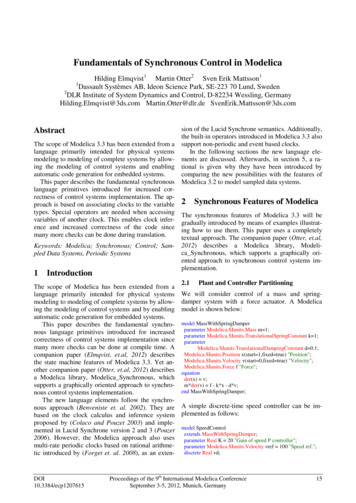
Session 1A: Hybrid Modelingreplicates a factor 5 times the value ofthe variable with the slower clock to have a clock afactor faster.The simulation results are shown below. Notethat xd and uOuter have a slower sample rate than uInner.superSampleIt is also possible to introduce sub-clocks that tick acertain factor slower than the base clock. Such subclocks are perfectly synchronized with the baseclock, i.e. the definitions and uses of a variable aresorted in such a way that when sub-clocks are activated at the same clock tick, then the definition isevaluated before all the uses.Such sub-clocks can, for example, be used to saveCPU resources. In some cases, an outer controller ofa cascade control architecture does not need to beevaluated as often as the inner controller.When using several clocks, it is convenient andclear to declare them. Modelica 3.3 introduces a newbase type, Clock, for this purpose:Clock cControl Clock(0.01);Clock cOuter subSample(cControl, 5);The subSample operator creates a clock which is a factor slower; in this case cOuter becomes 5 times slowerthan cControl. The subSample operator can also operateon a discrete-time variable and then picks the valueat every factor clock tick of the clock of this variable.Such clock variables can then be used as argumentto the sample operator:xd sample(x, cOuter);vd sample(v, cControl);The outer controller now calculates uOuter at the rateof cOuter. uOuter is the velocity reference, vref, for theinner controller which is compared to the sampledvelocity measurement, vd. vd has clock cControl, i.e., 5times faster than uOuter. Trying to directly calculateuOuter-vd would give a clocking error since the semantics is not clear. The user needs to state the intentby using a clock conversion operator. In this caseuOuter needs to be converted to the faster clock byusing the superSample operator:vref superSample(uOuter, 5);DOI10.3384/ecp12076152.4Interval of ClockIt is possible to inquire the actual interval of a clockby using the interval() operator. One example of theneed is when using difference approximations. Assume that no speed sensor is available and the speedneeds to be estimated from changes of position. Afirst order approximation is shown below. It uses afaster sampling of the position, x:Clock cFast superSample(cControl, 2);xdFast sample(x, cFast);vd subSample((xdFast-previous(xdFast))/interval(), 2);After approximating the derivative at the higher rate,the result is sub-sampled with a factor of 2 to get therequired rate of vd.2.5Phase of ClockTo better control the scheduling of calculations, it ispossible to shift the phase of a clock. For example,the calculation of the outer controller code will bedone before the inner controller code due to the dataflow. This might give jittering in the actuator signaluInner caused by the slight delay due to the computation time. One way to avoid this is to schedule theProceedings of the 9th International Modelica ConferenceSeptember 3-5, 2012, Munich, Germany17
Fundamentals of Synchronous Control in Modelicaouter code to be executed later in the cycle and toaccept the use of an old value of uOuter. This is accomplished in the following way:The simulation results are shown below. In particularit can be noted how uOuter is shifted 2/3 of the interval on uInner.Clock cOuter subSample(shiftSample(cControl, 2, 3), 5);The shiftSample operator shifts the clock a part of theinterval. In this case 2/3 of the interval of the clockcControl.By changing the clock cOuter in this way, the calculation of uOuter will be delayed and will not besynchronized to vd. This needs to be compensated byusing backSample which shifts the clock in the opposite direction to shiftSample:vref backSample(superSample(uOuter, 5), 2, 3);It should be noted that this means that a start valuemust be given to uOuter which is used before theclock of uOuter has started ticking.The complete model including all aspects discussed above is given below:model ControlledMassextends MassWithSpringDamper;parameter Real KOuter 10 "Gain of position PI controller";parameter Real KInner 20 "Gain of speed P controller";parameter Real Ti 10 "Integral time for pos. PI controller";parameter Real xref 10 "Position reference";discrete Real xd;discrete Real eOuter;discrete Real intE(start 0);discrete Real uOuter(start 0);discrete Real xdFast;discrete Real vd;discrete Real vref;discrete Real uInner(start 0);Clock cControl Clock(0.01);Clock cOuter subSample(shiftSample(cControl, 2, 3), 5);Clock cFast superSample(cControl, 2);equation// position sensorxd sample(x, cOuter);// outer PI controller for positioneOuter xref-xd;intE previous(intE) eOuter;uOuter KOuter*(eOuter intE/Ti);// speed estimationxdFast sample(x, cFast);vd subSample((xdFast-previous(xdFast))/interval(), 2);// inner P controller for speedvref backSample(superSample(uOuter, 5), 2, 3);uInner KInner*(vref-vd);// force actuatorf hold(uInner);end ControlledMass;An interesting question is when a clock starts to tick.In principal there are two useful approaches: A clockstarts ticking at time 0 seconds or it starts ticking atthe simulation start time (or when a device isswitched on). The synchronous extensions of Modelica use the second approach because from the viewof a hardware device, there is no absolute but onlyrelative time.Operator y shiftSample(u, c, r) defines a new clockthat basically shifts the first activation of the clock ofy in time c/r*interval(u) later than the first activation ofthe clock of u. This definition gives not a precisetime definition because interval(u) is of type Real. Furthermore, it only holds in special cases, such as forperiodic clocks with a fixed period. The precise timedefinition that holds for all clocks is achieved byconstructing (conceptually) a clock cBase:Clock cBase subSample(superSample(u, r), c);and the clock of y shiftSample(u, c, r) starts at the second clock tick of cBase and y is set to the most recently available value of u.In a similar way the operator y backSample(u, c, r)defines a new clock that basically shifts the first activation of the clock of y in time c/r*interval(u) beforethe first activation of the clock of u. Similarly toshiftSample, the precise time definition is achieved byconstructing (conceptually) a clock cBase :Clock cBase subSample(superSample(u, r), c);18Proceedings of the 9th International Modelica ConferenceSeptember 3-5, 2012, Munich GermanyDOI10.3384/ecp1207615
Session 1A: Hybrid Modelingand the clock of y backSample(u, c, r) is shifted a timeduration before the clock of u, such that this durationis identical to the duration between the first and second clock tick of cBase.The backSample(.) operator is more critical than theshiftSample(.) operator: The clock of v starts before theclock of u and therefore a start value for u is neededand before the first tick of the clock of u, the operatorreturns this start value. Additionally, there is the restriction that the clock of v cannot start before thesimulation start time.On first view, one could have only provided oneoperator to shift the start of a clock forward or backward in time. However, shifting backwards in timerequires providing a start value, whereas this is notthe case when shifting forward in time. Since theseare therefore structurally different cases, it is betterto use two different operators.2.6Exact Periodic ClocksIn the previous sections, periodic clocks are definedwith the Clock(period) constructor, where period is oftype Real and defines the sample period. The semantics is that two clocks of this kind are not time synchronized to each other. Example:Clock c1 Clock(0.1);Clock c2 superSample(c1,3);Clock c3 Clock(0.1/3);Clock c1 and c2 are precisely time synchronized toeach other and at every third tick of c2, clock c1 ticks.However, clock c3 is not time synchronized to c1 orc2 and there is no guarantee that c3 ticks at everythird tick of c1. The reason is that calculations withReal numbers are not exact and subject to small numerical errors.Alternatively, a periodic clock can be definedwith the Clock(c,r) operator, where c and r are of typeInteger, and the fixed sample period is defined as therational number c/r. The semantics is that all clocksdefined in this way are precisely time synchronizedto each other. Example:Clock c1 Clock(1,10);// period 1/10Clock c2 superSample(c1,3); // period 1/30Clock c3 Clock(1,30);// period 1/30Clocks c1, c2, and c3 are precisely time synchronizedto each other and at every third tick of c2 and of c3,clock c1 ticks.An interesting question is which periods can bedefined with exact periodic clocks? Basically, a period is defined as the quotient of two Modelica Integernumbers, which are usually 32 bit integers. Therefore, periods in the range 10-9 . 109 s can be directlydefined. However, clocks can be sub- and supersampled, e.g,DOI10.3384/ecp1207615superSample(Clock(1, 1000000000) , 1000000000);The resulting clock will have a period of 10-18 s. Inother words, from a Modelica point of view, any period that can be represented by a rational numberwith unlimited precision can be defined. In the Modelica 3.3 specification it is stated that “it is requiredthat accumulated sub- and super sampling factors inthe range of 1 to 263 can be handled”. Therefore, every tool should support internally at least 64 bit integers and therefore periods in the range 10-18 . 1018 s.2.7Clocked When ClauseAlthough the new synchronous operators allow defining clocked equations implicitly due to clock inference, it is sometimes still useful to explicitly define that a group of equations is associated with thesame clock. In order to not introduce yet another newkeyword, the already existing when-clause is overloaded for this purpose. Example:import Modelica.Utilities.Streams.print;equationwhen Clock(0.1) thenx A*previous(x) B*u;y C*previous(x) D*u;print("Clock ticks at time " String(sample(time)));end whenIf a clock is used in a when-clause then all equationsin the when-clause are associated with this clock. Insuch a case, the equations in the when-clause can bearbitrary equations (recall that for standard whenclauses with a Boolean condition, all equations in thewhen-clause must have a variable reference on theleft hand side of every equation, i.e., equations mustbe of the form “x expr”).In the example above, all three equations in thewhen-clause belong to the same partition that is areassociated to clock Clock(0.1). When-clauses might beused to clearly define that equations are associatedwith the same clock. Furthermore, there are exceptional cases as in the example above, where it wouldbe not possible to associate the print(.) statement toClock(0.1) without a when-clause because no variableof the clocked partition is used in the print statement.If the clock of the when-clause is defined somewhereelse and shall be deduced by clock inference, thenthe clock Clock() needs to be used in the when-clause:when Clock() then// clock is inferredx A*previous(x) B*u;y C*previous(x) D*u;print("Clock ticks at time " String(sample(time)));end whenIn Modelica 3.3, clocked when-clauses are restricted:The condition must be a clock (and not, say a Boolean expression of clocks such as “c1 or c2”), an else-Proceedings of the 9th International Modelica ConferenceSeptember 3-5, 2012, Munich, Germany19
Fundamentals of Synchronous Control in Modelicawhen part is not allowed, and the clocked whenclause can only appear in an equation section.2.8Varying Interval ClocksIt is also possible to define clocks with a varyinginterval between the sampling points. As an example, considermodel VaryingClockInteger nextInterval(start 1);Clock c Clock(nextInterval, 100);Real v(start 0.2);Real d interval(v);Real d0 previous(nextInterval)/100.0;equationwhen c thennextInterval previous(nextInterval) 1;v previous(v) 1;end when;end VaryingClock;As the plot shows, vs3 samples each third point of v.We can also super-sample:Real vS5 superSample(v, 5) ;Real dS5 interval(vS5);It defines a Clock c with varying interval, nextInterval.A definition of the formClock c Clock(nextInterval, 100)states that clock c ticks at the simulation start andthen every nextInterval/100 seconds, and at every clocktick, nextInterval can be newly computed. Since at thefirst clock tick, previous(nextInterval) is equal to thestart value of nextInterval ( 1), the value of nextIntervalat the first clock tick is 1 1 2, and therefore thesecond clock tick is at 2/100 seconds. The furtherticks are at 5/100, 9/100 etc. The behavior of the variable v is shown in the following plot:The 5 super-sampling points are evenly distributed intime within the intervals of clock c as shown by theplot of dS5. Let us now sub-sample dS5:Real vS5s3 subSample(vS5, 3) ;Real ds3S5 interval(vs3S5);The variables d interval(v) andd0 previous(nextInterval)/100.0 are equal.Let us sub-sample v by adding to the model:Real vs3 subSample(v, 3) ;Real ds3 interval(vs3);20The result is that vS5s3 is every third sample of vS5resulting in a more irregular sampling interval. Theequation vS5s3 subSample(vS5, 3) can be expanded asvS5s3 subSample(superSample(v, 5), 3).What is the result if we do it in the reverse order,vs3S5 superSample(subSample(v, 3), 5)? For the clock c,the time to the next tick is known at the current tick.Proceedings of the 9th International Modelica ConferenceSeptember 3-5, 2012, Munich GermanyDOI10.3384/ecp1207615
Session 1A: Hybrid ModelingHowever, this is not the case for the clock of subSample(v, 3). The interval to its next tick is the sum of 3future intervals of c and only the first term is known.The definition of super-sampling does not require theintervals of super-sampling to be equidistant in time.The definition is instead based on counting ticks. Itmeans that vs3S5 vS5s3.In Modelica, a non-periodic clock can only be introduced by using an explicit clock constructor. Thefactors of sub-sampling or super-sampling must beparameter expressions, which mean that neither subsampling nor super-sampling can construct a clockwith varying interval from a periodic clock. It is alsorequired that there must be only one clock constructor, c, in the same base-clock partition if c is a nonperiodic clock. All this means that we can construct anew clock c0 that is a super-sampled clock of c, suchthat all other clocks can be modeled as pure subsampling clocks of c0. As we have described, thereare no issues in making a faster clock c0 by supersampling c. The sub-sampling of c0 to implement allthe sub-clocks is then just a matter of counting ticksand picking the nth samples.2.9Boolean ClocksIt is also possible to define clocks that tick when aBoolean expression changes from false to true. Forexample assume that a clock shall tick whenever theshaft of a drive train passes 180o. This can be definedas (Otter, et.al. 2012):w der(angle);J*der(w) tau;when Clock(angle hold(offset) Modelica.Constants.pi) thenoffset sample(angle);end when;At the simulation start the discrete variable offset hasa start value of zero. Therefore, the first clock tickappears when angle becomes larger as 180o. Then,offset is set to the actual angle, and the next clock tickappears at another full rotation of the shaft. Note,that the Boolean expression is continuous-time, andtherefore the clocked variable offset cannot be directly used, but must be casted from a clocked to a continuous-time variable with operator hold. A typicalsimulation result is shown in the next figure:Operators subSample, superSample, shiftSample and backcan also be applied on Boolean clocks. However, there are restrictions. For example, superSample(.)cannot introduce new ticks because the next clocktick is not known in advance. Example:SampleClock u Clock(sine(time) 0);Clock y1 subSample(u,4);Clock y2 superSample(y1,2); // fine y2 subSample(u,2)Clock y3 superSample(u, 2); // error2.10 Discretized continuous timeA partition (i.e., a set of equations) that is marked bysample, hold, subSample, superSample etc. operators iscalled a “clocked partitions”. There are two differentkinds of clocked partitions:Clocked discrete-time partitionThis is the type of partition discussed so far, consisting of algebraic equations, potentially using operators previous(.) and interval(.) in the equations.Clocked discretized continuous-time partitionThis is a partition where the operator der(.) is used(and then previous(.) and interval(.) must not be present). In such a case a set of differential and algebraic equations is marked to be a clocked partition. Thesemantics is that at clock ticks these equations aresolved with a specified integration method from theprevious to the next clock tick. The integrator forsuch a partition is propagated (inferred) similarly asa clock and therefore it suffices to define it at a fewplaces.This is a powerful feature since in many cases it isno longer necessary to manually implement discretetime components but it suffices to just build-up acontroller with continuous-time components andthen sample the input signals and hold the outputsignals.In the following example a continuous-time PIcontroller that gets a reference and a measurementsignal as input is automatically transformed to aclocked partition:model ClockedPIparameter Real k;parameter Real T;input Real y ref;input Real y mes;output Real u(start 0.0);discrete Real e;discrete Real x;discrete Real ud;Clock c Clock(Clock(0.1), solverMethod "ImplicitEuler");equation// Sampling the inputse sample(y ref,c) - sample(y mes);DOI10.3384/ecp1207615Proceedings of the 9th International Modelica ConferenceSeptember 3-5, 2012, Munich, Germany21
Fundamentals of Synchronous Control in Modelica// PI controllerder(x) e/T;ud k*(x e);first tick of the clock of u, the start value of u isreturned.// Holding the outputu hold(ud);end ClockedPI;With the declaration Clock(c, solverMethod), the solverMethod (defined as String) is associated to clock c andthe partitions to which this clock is associated aresolved with the specified solver method ( integration method). As already mentioned, this feature canbe used to discretize continuous-time blocks. Also,nonlinear plant models can be inverted and the inverse model can be discretized and used, say, asfeedforward controller part in a sampled data controller, see (Otter, et. al. 2012). Furthermore, thisfeature can be utilized for multi-rate real-time simulations where a model is partitioned in different partsand these parts are solved with different integrationmethods and step sizes.3Synchronous OperatorsAll newly introduced operators of the synchronousextension to Modelica have been sketched so far. Inthis section, a short overview of these operators isgiven:Clock ConstructorsClock(): Returns a clock that is inferredClock(i,r): Returns a variable interval clock where thenext interval at the current clock tick is definedby the rational number i/r. If i is parameteric,i.e., a literal, a constant, a parameter or an expression of those kinds, the clock is periodic.Clock(ri): Returns a variable interval clock where thenext interval at the current clock tick is definedby the Real number ri. If ri is parametric, theclock is periodic.Clock(cond, ri0): Returns a Boolean clock that tickswhenever the condition cond changes from falseto true. The optional ri0 argument is the valuereturned by operator interval() at the first tick ofthe clock.Clock(c,m): Returns clock c and associates the solvermethod m to the returned clock .Base-clock conversion operatorssample(u,c): Returns continuous-time variable u asclocked variable that has the optional argumentc as associated clock.hold(u): Returns the clocked variable u as piecewiseconstant continuous-time signal. Before the22Sub-clock conversion operatorssubSample(u,factor): Sub-samples the signal or clock uby the integer factor. If factor is not present, it isinferred.superSample(u,factor): Super-samples the signal or clocku by the integer factor. If factor is not present, it isinferred.shiftSample(u,c,r): Shifts the clock of a signal or clock uforward in time.backSample(u,c,r): Shifts the clock of a signal or clock ubackward in time. Before the first tick of theclock of u, the start value of u is returned.Other operatorsprevious(u): At the first tick of the clock of u, the startvalue of u is returned. At subsequent clockticks, the value of u from the previous clock activation is returned.interval(u): Returns the interval between the previousand the present tick of the clock to which signalu is associated. The interval is returned as a Real number.4Base-clock and Sub-clockPartitioningConsider the example SpeedControl in section 2.1. Thevariables and equations of MassWithSpringDamper forma well-defined continuous-time model together withthe equation f hold(u) from SpeedControl if we view uas a known input. Similarly the variables and equations added in SpeedControl when extending fromMassWithSpringDamper form a well-defined discretesystem if we disregard the equation f hold(u), whichalready is used in the continuous time system and ifweview v,referredin the equationvd sample(v, Clock(0.01)) as a known input. We havenow decomposed the system in a continuous-timepartition and in a discrete-time partition.For the general case, we observe that the sampleand hold operators serve an important role as identifying the interfaces between the two kinds of partitions. The first argument of sample identifies inputs todiscrete-time partitions that must be provided bycontinuous time partitions. Similarly the first argument of hold identifies inputs to continuous-time partions that must be provided by discrete-time partitions. If the first arguments are expressions, auxiliaryvariables are introduced.Proceedings of the 9th International Modelica ConferenceSeptember 3-5, 2012, Munich GermanyDOI10.3384/ecp1207615
Session 1A: Hybrid ModelingThe idea of the base-clock decomposition
the state machine features of Modelica 3.3. Yet an-other companion paper (Otter, et.al, 2012) describes a Modelica library, Modelica_Synchronous, which supports a graphically oriented approach to synchro-nous control systems implementation. The new language elements follow synchro- the nous approach (Benveniste et. al. 2002). They are