Transcription
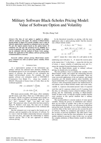
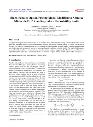
FX OPTION PRICING: RESULTS FROM BLACK SCHOLES,LOCAL VOL, QUASI Q-PHI AND STOCHASTIC Q-PHI MODELSKrishnamurthy Vaidyanathan1AbstractThe paper suggests a new class of models (Q-Phi) to capture the informationthat the market provides through the 25-Delta Strangles and 25-Delta Risk Reversals.The model is able to capture the stochastic movements of a full strike structure ofimplied volatilities.We argue that extracting information through this model andpricing path-dependent and non-benchmark strike options is a better methodologythan using a contant implied volatility. The model can be used to price exotic optionsand hedge them robustly with benchmark European options.1IntroductionPricing derivative products is about computing the right probabilities. Forinstance, for a foreign exchange vanilla option, we need to know the probabilitydensity function of the underlying exchange rate at maturity. This allows calculatingthe probability that spot at maturity is within a given interval, which for Call optionsis greater than strike and for Put options is less than strike. For a barrier option, weneed to compute the joint probability that the exchange rate is within a given intervalat maturity and that the spot did not touch the barrier on its path from option start dateto maturity. Next we would multiply the appropriate probabilities with the payoff ofthe option and sum over over all possible outcomes of the exchange rate at maturity toget the expected payoff. The options value is this payoff discounted to the option startdate.We imply the probabilities from market prices, which for liquidly tradedoptions is implied volatility. The implied volatility varies for different option strikes.The benchmark strikes that get traded in the foreign exchange options are 50-delta(more commonly known as at-the-money-forward or ATMF strike), 25-Delta Call and25-Delta Put (also known as 75-delta Call). Figure 1 depicts a typical volatility smilequoted in the market. The market quotes ATMF volatility (or short form ‘vol’) , 25Delta Strangle and 25-Delta Risk Reversal which are related to the 25-Delta Call andPut volatilities as follows:25-Delta Strangle (25-Delta Call vol 25-Delta Put vol)/2 – ATMF vol25-Delta Risk Reversal 25-Delta Call vol - 25-Delta Put vol (favouring Calls)(1)(2)Alternatively, if 25-Delta Put vol is higher than 25-Delta Call vol, 25-DeltaRisk Reversal is said to be ‘favouring Puts’ and is quoted as (25-Delta Put vol - 25Delta Call vol).1SINE, CSRE Building, IIT Bombay, Powai, Mumbai – 400076. India.E-Mail: vaidyanathan@alumni.iitk.ac.in1
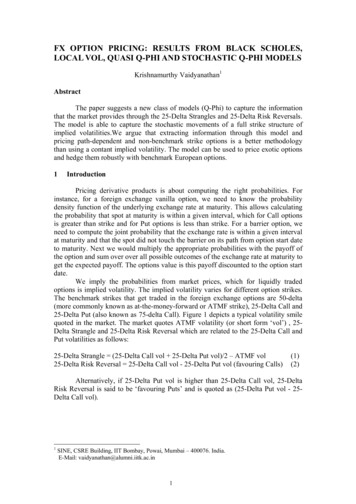
18.00%25-Delta Call,17.00%Volatility SmileImplied 00%ATM F, 13.50%13.00%0%25%50%Strike delta75%Fig. 1. The figure depicts the volatility smile that traders quote for liquid foreignexchange options. The benchmark strikes correspond to 25-Delta-Call, ATMF i.e. 50Delta and 25-Delta-Put.1.1Problem of multiple volatility for same underlyingEuropean options are often priced and hedged using the Black-Scholes (BS)model. In BS model there is a one-to one relation between the price of a Europeanoption and the volatility parameter σBS . Consequently, option prices are often quotedby stating the implied volatility σBS , the unique value of the volatility which yieldsthe option’s dollar price when used in BS. In theory, the volatility σBS in BS model isa constant. In practice, options with different strikes K require different volatilitiesσBS to match their market prices as shown in figure 1. Handling these market skewsand smiles correctly is critical to foreign exchange desks, since they usually havelarge exposures across a wide range of strikes. Yet the inherent contradiction of usingdifferent volatilities for different options makes it difficult to successfully managethese risks using BS model.1.2The information content of benchmark options prices.There are good reasons for incorporating the prices of benchmark optionprices like 25-Delta Strangles and 25-Delta Risk Reversals into a model for pricingand risk managing foreign exchange options. Since the advent of the famous Blackand Scholes (1973) option pricing model and the introduction of foreign exchangeoption contracts, the volume and liquidity of fx options has increased exponentially.Simultaneously more and more complex, exotic option specifications have arisen withfeatures ranging from knock-in and knock-out barriers, digital options and rangebinaries to combinations of these and other features with many different payofffunctions.While on the one end of the spectrum the development has gone towardsincreasingly complex specifications, there has been a significant increase in liquidityin the markets of standard European Call and Put options. For almost every exchangerate, there are liquid markets for European options with a broad range of maturitiesand strike prices – in particular the strikes corresponding to 25-Deltas. Thesebenchmark options make the trading of a new piece of information possible information on volatility.2
The option prices contain fundamental information on not just the volatilitybut also other information like the co-movement of volatility with the underlying. Forinstance, when the market puts a higher premium on 25-Delta Puts vis-à-vis 25-DeltaCalls, it is implicitly stating that it expects the volatility to be higher when spot goeslower than the case when spot goes higher. Therefore a high risk-reversal implies ahigh correlation between Spot and Volatility. Similarly, a high strangle implies thatthe market expects volatility itself to be volatile. As an aside, if volatilities were notvolatile, the options market may not exist!Given that the benchmark option prices reveal additional information aboutthe likely dynamics of the underlying, a pricing model should use their prices as input.This should yield an increase in accuracy over the standard Black-Scholes model.Then the standard options can also be used as additional hedge instruments.The model presented here tries to take these points into account. It is designedto incorporate benchmark option prices and thus the information that they contain, inorder to improve the pricing of more exotic instruments.1.3Related LiteratureThe deviation of observed market prices for options from their theoreticalcounterparts as given by the Black-Scholes formula has triggered a large literature inwhich both academics and practitioners alike have tried to improve on the limitationsof the Black Scholes model.One strand of the literature concentrates on the implied tree approach. The aimis to keep as closely as possible to the Black-Scholes setup while exactly reproducingthe option prices given in the market. This is achieved by specifying a time and statedependent volatility function which does not contain any additional randomcomponent. Models of this type are by Rubinstein (1995), Derman and Kani (1994),Derman et.al. (1996) and Dupire (1994).While exactly reproducing the option prices observed in the market theimplied volatility models have the drawback that they do not allow for idiosyncraticstochastic dynamics in the option prices. This is in conflict with empirical observationand with the continuous updating of the new information reflected in the optionprices. The poor results in a hedging test performed by Dumas et.al. (1999) areprobably also due to this drawback. Dupire (1996) took a first step towardsincorporating stochastic dynamics into the term structure of volatilities, but again hemodels realized volatilities and forward contracts on it, and not implied volatilitiesfrom options prices.Derman and Kani (1998) extended their implied tree approach to allow forstochastic dynamics in the full term and strike structure of implied local volatilities.They derive restrictions on the drift of the local volatilities that are necessary forabsence of arbitrage, and these restrictions involve integrals over all possibleunderlying prices and times before the maturity of the forward volatility concerned.The complexity of these restrictions makes the model hard to handle and we are goingto propose a slightly different approach. Furthermore it is not obvious how in Dermanand Kani’s model it is ensured that the implied volatilities satisfy certain no-arbitragerestrictions as expiry is approached. The fundamental problem is, that Derman andKani specify two things that may be contradictory: the dynamics of the spot volatilityand the implied volatilities for different strike prices and maturities.The development of local volatility models by Dupire (1994), and DermanKani (1996) was a major advance in handling smiles and skews. Local volatility3
models are self-consistent, arbitrage-free, and can be calibrated to precisely matchobserved market smiles and skews. Currently these models are still used for managingsmile and skew risk. However, the dynamic behavior of smiles and skews predictedby local vol models is exactly opposite of the behavior observed in the marketplace:when the price of the underlying asset decreases, local vol models predict that thesmile shifts to higher prices; when the price increases, these models predict that thesmile shifts to lower prices. In reality, exchange rates and market smiles move in thesame direction. This contradiction between the model and the marketplace tends tode-stabilize the delta and vega hedges derived from local volatility models, and oftenthese hedges perform worse than the naive Black-Scholes’ hedges.We will follow an approach for modeling fundamental quantities like thestochastic process of the volatility of the underlying as in the traditional stochasticvolatility models of Hull (1987), Heston (1993) or Stein and Stein (1991). Thisfacilitates the fitting of the model to observed option prices and gives the model alarger degree of flexibility.Using a model based approach means that we do not use the market-basedapproach applied to the term structure of implied volatilities which is similar to themarket models of the term structure of interest rates by Miltersen, Sandmann andSondermann (1995), Brace, Gatarek and Musiela (1997) and Jamshidian (1997). Nordo we model the instantaneous conditional forward volatilities as in the effectivevolatility model by Derman and Kani (1998), or forward variances like in Dupire(1992) or model the Black-Scholes implied volatilities.Another direction of research has been on the nature of the underlying priceprocess which was assumed to be a lognormal Brownian motion by Black andScholes. Well known papers of this approach are by Hull (1987), Heston (1993), orStein and Stein (1991) as discussed earlier.The approach taken here draws upon both the strands of research thus far. Wemodel the instantaneous volatility of exchange rates rather than implied volatilities asin the market models. We also incorporate stochasticity in the underlying volatilityi.e. volatility of the underlying is assumed to be uncertain as is observed in themarket.Some of the constraints of our model are that though they reproduce thetypical shapes of implied volatilities observed in the markets known as the smile, theyneed to be calibrated to the benchmark options, i.e. they are computationally intensiveand there is no closed form solution for calculating option price. Another constraint isthat this model has only one additional factor driving the stochastic volatility andcannot be extended to the multi-factor case.In what follows we briefly present the models that are currently used inforeign exchange options: the famous Black-Scholes model, the Q-Φ model and theStochastic Q-Φ model, and compare the results obtained from each of these models.4
2The Black-Scholes ModelWe first introduce the Black-Scholes Model2.1Spot Dynamics and the Local VolatilityThe Black-Scholes (1973) approach towards the probability density isstraightforward. The basic assumption is that the exchange rate follows a lognormalstochastic process:dS t µ * dt σ * dWt(3)StThe Lognormal Stochastic riftdt99.9899.97012345678910time in daysFig. 2. The Lognormal Stochastic Process. The blue line shows a simulated path forthe first 10 days of an exchange rate according to equation (3). Initial spot S0 100,volatility σ 10% and drift µ 1%. The pink line shows the drift only, i.e. thedeterministic part of equation (3). The double-arrows indicate the size of the spotmove dS in the second time step.The relative move of spot dSt/St over the next time interval dt is given by adeterministic part, the so-called drift term µ*dt and a random term σ*dWt . The driftterm is given by the difference of the numeraire and asset interest rates: µ*dt (rnum –rass)*dt. The random part is driven by dWt ε * dt , where ε is a random numberthat is drawn from a standard normal distribution N(0,1). The model parameter thatgoverns the dynamics of the Black-Scholes model is the local or instantaneousvolatility σ .We are interested in the distribution of spot at maturity of the option. So weperform a Monte Carlo simulation to create it. Draw a random number ε from ourstandard normal distribution N(0,1), plug it into equation (3) and determine the newspot St 1 St dSt, which is the starting point for the next time interval dt. If werepeat this procedure until we reach the expiry date of the option we generate a singlerandom path of spot from today’s date to expiry date. A knockout barrier is taken intoaccount by stopping any path that touches this level. The information of the outcome5
of St for many paths created in the same way provides us with a frequency distributionof outcomes of spot at expiry. After normalisation, i.e. division by the number oflaunched paths, we obtain the probability distribution of spot at expiry.2.2The Implied or Black-Scholes VolatilityIn a Black-Scholes world, instead of running a tedious Monte Carlo simulationwe can directly solve the stochastic partial differential equation (3)2 σ BS t σ BS Wt (4)S t S 0 * exp µ 2 Equation (4) allows jumping a macroscopic time step t, e.g. t expiry date,rather than only microscopic steps of the size dt. σBS is the implied or Black-Scholes2volatility. As ε is from N(0,1), σ BSWt σ BS ε t is distributed N (0, σ BSt ) , i.e.normally distributed with standard deviation σ BS t and zero mean. Taking thelogarithm of equation (4) shows why the Black-Scholes model is also known as thelognormal model.2 St σ BS t σWt ln µ (5)2S 0 Equation (5) tells us that ln(S t S 0 ) is normally distributed with mean22µ σ 2 and standard deviation σ BS t , i.e. N (µ σ BS2 , σ BSt ) . A simpletransformation results in the PDF of St . The Black-Scholes or implied volatility σBS isa tenor volatility whereas σ is only valid for the next infinitesimal time step. In theBlack-Scholes world these two volatilities numerically agree, i.e. σ σBS , however,these volatilities are two different parameters as will become more evident when weconsider more sophisticated models.The derivation of the PDF of St given that the spot did not touch the barrier onits path is a bit more cumbersome but the point to be made is that we arrive at aprobability density function for spot at maturity using a single model parameter σ.2BS2.3CalibrationThe calibration of the Black-Scholes model is simple. We determine σBS ( σ)such that the Black-Scholes price of an option is equal to the market price of thisoption. The standard practice in the market is to choose ATMF (at-the-moneyforward) and 25-Delta Call and Put strike options for calibration.2.4PricingPricing in the Black-Scholes world is simple too. For most option products wecan provide an analytical formula for the integral of the product of probability timespayoff. This makes implementation of the algorithms fast and robust.2.5No SmileFor a given tenor the volatility smile is defined as the implied volatility as afunction of strike. Thus, per construction, the Black-Scholes model does not exhibitany smile, i.e., the function σBS(K) σBS is constant.6
33.1The Q-Φ ModelSpot Dynamics and the Local VolatilityThe Q-Φ model allows for interest rates and hence the drift term to be timedependent. More importantly, however, the local volatility is assumed to depend onspot and time.dS t µ (t ) * dt σ (S , t ) * dWtSt(6)Some Wall Street houses incorporate this temporal information in order toprice path-dependent options. However, the dependence of implied volatility on thestrike, for a given maturity known as the Smile effect, is trickier. Many researchershave attempted to enrich the Black-Scholes model to compute a theoretical smile.Unfortunately they have to introduce a non-traded source of risk, jumps in the case ofMerton (1976) and stochastic volatility in the case of Hull and White (1987), thuslosing the completeness of the model. Completeness is of high value since it allowsfor arbitrage pricing and hedging.If we look carefully, the process in the equation above looks very similar tothe lognormal process of the Black-Scholes model that we introduced in equation (3).Yet as we simply allow the local volatility to depend on spot and time we are able tocapture today’s volatility smile. For option pricing we could again recourse to theMonte Carlo technique as described before for the Black-Scholes model. Draw arandom number ε from N(0,1), plug it into equation (6) and determine the new spotSt 1 St dSt. However, to do so, we require the values of the local volatility foreach attainable time and spot level, the so-called local volatility surface.3.2The Local Volatility SurfaceThe Q-Φ model does not provide an analytic function for σ(S,t). Rather wecan derive an equation that relates the local volatility to the derivatives of the optionprices with respect to strike and time. C C µ (T ) * K *rass (T ) * C K T(7)σ 2 (K , T ) 2 C12*K *2 K 2where C denotes the price of a Call option with tenor T and strike K. If we knewoption prices for all tenors and strikes, we could numerically work out the derivativesin equation (7) and determine the local volatilities. In fact, this is the route that istaken.Obviously, we need to know how the Q-Φ model computes vanilla optionprices. They are computed as the average of two Black-Scholes prices.1(8)C (BS (σ 1 ) BS (σ 2 ))2BS( ) denotes the Black-Scholes option pricing formula and the two impliedvolatilities are given by7
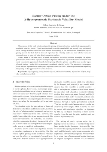
F σ 1 σ ATMF (T ) * 1 m Q (T ) Φ(T ) * ln (9) K Equation (8) and (9) can be interpreted in a simple way: The Q-Φ modelassumes a two-point distribution for volatility. For a given strike K the volatility willbe either σ1 or σ2 with probability 1/2. The meaning of the model parameters Q and Φis explained later.23.3CalibrationWe calibrate the model against the market prices for three options, ATMF, 25delta Calls and Puts. We have to fit the three parameters of the model, σATMF, Q, andΦ, such that the Q-Φ prices i.e., equation (8) match the market prices. Using equations(8) and (9) yields vanilla option prices for all tenors and strikes and equation (7)providesuswiththevolatilitysurface.Local Volatility 125.00.00%162time in dayssigma20.00%spotFig. 3. Q-Φ Local Volatility Surface as a Function of Time and Spot. The graph aboveis generated with the Q-Φ model. It shows a 6M local volatility surface. We use aninitial spot of S0 100, 6M ATMF volatility σATMF 13.5%, strangle Str 0.5% andrisk reversal RR 2% for Puts. The calibration returned Q 0.36 and Φ -1.21.3.4PricingThe volatility surface is fed into a Monte Carlo simulation or a finitedifference grid to price exotic options consistent with the vanilla market. Apart fromvanilla options, for which we can recourse to equation (8) there is no analyticalsolution for Q-Φ option prices.3.5The Use of the Wrong NumberThe implied volatility is the parameter that we have to plug into the BlackScholes formula to obtain the market price of an option. For the Q-Φ model there isno obvious connection between the local volatility and this implied volatility. The8
local volatility surface contains the full information about today’s smile. We can usethis surface to correctly and consistently price any vanilla or exotic option. Theimplied volatility, in contrast, is simply the wrong number to be put into the wrongformula to get the vanilla prices right. However, using the knowingly wrong BlackScholes formula allows market participants to express the smile in a standardised wayin two single numbers: the strangle and the risk reversal.3.6SmileWe can easily relate Q and Φ to strangle and risk reversal. As we will show Φintroduces some asymmetry to the model while Q creates a symmetric smile.A positive Φ tends to increase both, σ1 and σ2 and for options with K F, i.e.OTM calls, and decreases both for options with K F. Thus a positive Φ correspondsto a risk reversal that favours calls. Obviously, Φ does not have any impact on theprice of ATMF options as ln(F K ) in equation (9) vanishes in that case.Equation (8) and (9) show that Q does not affect the price of an ATMF optionwhile it does so for an OTM option. Look at an option’s Vega to understand thisresult. Vega as a function of volatility is fairly constant for ATMF options, i.e. ATMFoptions have zero Vomma2. In other words, the price of an ATMF option is an almostlinear function of volatility and we haveATMF:C 1 2 * (BS (σ 1 ) BS (σ 2 )) BS (1 2 * (σ 1 σ 2 )) BS (σ ATMF )In contrast, for OTM options Vega increases with rising volatility, i.e. theyhave positive Vomma. Alternatively, we say that the price of an OTM option is aconvex function3 of volatility. Thus forOTM:C 1 2 * (BS (σ 1 ) BS (σ 2 )) BS (1 2 * (σ 1 σ 2 ))Apparently, Q makes OTM options more expensive, that is, Q can be related tothe strangle.2Vomma is the second derivative of the options price C with respect to volatility C σ , itdescribes the curvature of the options price as a function of volatility.3For a convex function c we have (c( x ) c( y )) 2 c(( x y ) 2 )229
4The Stochastic Q-Φ modelWe provide the formulation and dynamics of the stochastic Q-Φ model.4.1Spot and Volatility DynamicsThe Stochastic Q-Φ model assumes the following dynamics for the exchangerate.dS t µ (t ) * dt σ t * f (S t , t )* dWtStdσ t ξ (t ) * dZ t(10a)(10b)σtwhereand2 S α (t ) Sf (S t , t ) 100 * β (t ) * 1 S0 S0 dZ t κ * dtwith κ N (0,1)The random term for the exchange rate in equation (10a) is similar to the onethat we have seen in the Q-Φ model. Here, the analytical function σ t * f (S t , t )determines the local volatility surface. However, in the stochastic model the volatilityitself is a random process with no drift and a volatility (of volatility) ξ .The model has four parameters: σ 0 , α , β , and ξ . σ 0 is the initial value forthe volatility. We will understand the meaning of the other parameters in whatfollows.We use the Monte Carlo approach to investigate on the dynamics of equations(10a) and (10b). We first draw a random number ε , plug it into equation (10a) todetermine the spot after the first time step S t 1 S t dS t . Before continuing with thenext time step, however, we have to draw a random number κ , plug it into equation(10b) to obtain the correct parameter σ t 1 σ t dσ t to be used for the second timestep and so on. As far as the local volatility surface is concerned, the Q-Φ model isfully deterministic. In contrast, in the stochastic Q-Φ model we can only predict thelocal volatility for an arbitrary point in the future in a probabilistic sense. We couldsay that the stochastic volatility process in equation (10b) vibrates the deterministicfunction σ t * f (S t , t ) in a random manner. Note that this isn’t exact in a mathematicalsense but it is a useful way of looking at the mechanics.We approach the full complexity of the model by first considering two specialcases of the stochastic Q-Φ model, the Quasi Q-Φ model (ξ 0) and the purelystochastic model (β 0) .4.2The Quasi Q-Φ ModelSuppose that the volatility of volatility vanishes (ξ 0) . This means thatvolatility itself is not a random variable. In this case the smile is fully deterministic.The local volatility surface is given by σ t * f (S t , t ) . The model becomes similar to the10
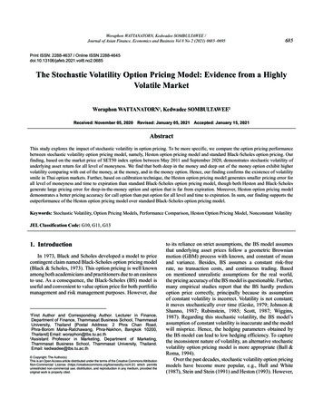
Q-Φ approach (Compare equations (6) and (10a)). The strangle is reflectedin β which creates a parabolic, symmetric local volatility surface around spot. Theasymmetry of the smile, i.e. the risk reversal, is created by α . We have to calibrateσ 0 , α , and β such that the market prices of three options, ATMF, 25 Calls andPuts, are matched.Local Volatility 3091.259103.887101.9time in days0.00%spotFig. 4. Stochastic Q-Φ Local Volatility Surface. The graph above is generated withthe stochastic Q-Φ model with vanishing volatility of volatility (ξ 0) . For theexample we used an initial spot of S 0 100 , 6M ATMF volatility σ ATMF 13.5% ,Str 0.5% andRR 2% for Puts. The calibration returnedstrangleσ 0 12.67% , β 0.27 and α 1.35 .4.3Q-Φ versus Quasi Q-Φ modelCompare the graphs of the local volatility in figures 3 and 4. Both surfaceswere fitted to the same smile. In spite of the fact that they appear to be very differentthere is no contradiction here. The local volatility surface is not directly observable inthe market. Rather the surface is implied and interpolated from three marketobservations only, the prices of a 6M ATMF option and a 6M 25 Call and Put. Infact the two models agree on the prices of these three options using the respectivelocal volatility surfaces. This is a trivial result as this is simply an inversion of thecalibration process. To understand in which case the models would give differentresults, consider the earlier Monte Carlo simulation exercise. Each path starts at t 0 ,i.e. at the front of figure 3 or 4 and runs in a random zigzag line to the back of thegraph. Along its way we pick up local volatilities and apply them to calculate the nextrandom shock for the spot. Consider a one-touch option. A path set out to run on thesurface of figure 3 presumably experiences a different probability to touch the triggerthan a path running on the surface of figure 4. To summarise, two different modelswill naturally agree on the prices of the vanilla products that are used for thecalibration. But they may give different answers, albeit the difference may be small,11
for products with different payoff functions, in particular path dependent options,such as knockouts and one touch options.4.4Pure Stochastic ModelAssume next that β 0 but ξ 0 . In this case the risk reversal is stillcreated by α . The strangle, however, is created by the stochastic nature of thevolatility. In our simplified picture of the stochastic model the local volatility vibrateswith an intensity proportional to the volatility of volatility. Thus, products withpositive Vomma, such as OTM options, will become more expensive. Accordingly,the deterministic volatility surface has a nonzero slope to account for the risk reversalbut does not exhibit any curvature (see figure 5). We have to calibrate σ 0 , α , and ξto the usual set of market prices: ATMF, 25 Calls and Puts.Local Volatility 3.180.0281.53091.259116.00.00%87101.9time in daysspotFig. 5. Stochastic Q-Φ Local Volatility Surface. The graph above is generated withthe stochastic Q-Φ model with vanishing β with similar parameters as before. Thecalibration returned σ 0 12.68% , and α 2.22 , and ξ 93% .4.5Purely Stochastic versus Quasi Q-ΦWhat are the differences between the purely stochastic model and the QuasiQ-Φ model. To work one out, we put ourself at the starting point of a Monte Carlosimulation, i.e. at t 0 and S 0 100 . Suppose that after a short period of time, say, acouple of days, the random shocks bring spot down to 95. We consider the view onthe volatility surface ahead with spot at 95. For the surfaces in figure 4 the landscapewill be tilted, i.e. the Quasi Q-Φ model increases the risk reversal when spot movesdown. In contrast, the slope of the surface in figure 5 remains unchanged, i.e. thestochastic model predicts that the risk reversal does not change at all.Another major difference is due to the nature of the purely stochastic model.As mentioned above, due to the stochastic nature of volatility the model will mark upall positive Vomma products. In contrast, the Quasi Q-Φ model assumes a12
deterministic, i.e. static local volatility. It cannot capture the benefit of positiveVomma. As an example, the price of a range binary will be higher if the purelystochastic model is used as compared to the Quasi Q-Φ model.4.6Stochastic Q-Φ or The MixAs described above, we either generate a smile by means of a purelydeterministic local volatility surface or we use a deterministic risk reversal combinedwith a stochastic volatility process. Both approaches are consistent with the market,i.e. ATMF, 25 Calls and Puts, so we cannot determine which approach is thecorrect one. Additional market information is required to find the most appropriatemodel.A purely deterministic volatility surface entails that the risk reversal changesquickly when spot moves, whereas in a purely stochastic model the smile sh
pricing path-dependent and non-benchmark strike options is a better methodology than using a contant implied volatility. The model can be used to price exotic options and hedge them robustly with benchmark European options. 1 Introduction Pricing derivative products is about computing the right probabilities. For