Transcription
International Journal of Economics and Finance; Vol. 8, No. 3; 2016ISSN 1916-971XE-ISSN 1916-9728Published by Canadian Center of Science and EducationEmpirical Performance of Black-Scholes and GARCH Option PricingModels during Turbulent Times: The Indian EvidenceAparna Bhat1 & Kirti Arekar11K. J. Somaiya Institute of Management Studies and Research, Mumbai, IndiaCorrespondence: Aparna Bhat, K. J. Somaiya Institute of Management Studies and Research, Vidyavihar,Mumbai – 400 077, India. Tel: 91-22-6728-3028. E-mail: aparnabhat@somaiya.eduReceived: December 21, 2015Accepted: January 13, 2016Online Published: February 25, 2016doi:10.5539/ijef.v8n3p123URL: hange-traded currency options are a recent innovation in the Indian financial market and their pricing is asyet unexplored. The objective of this research paper is to empirically compare the pricing performance of twowell-known option pricing models – the Black-Scholes-Merton Option Pricing Model (BSM) and Duan‟sNGARCH option pricing model – for pricing exchange-traded currency options on the US dollar-Indian rupeeduring a recent turbulent period. The BSM is known to systematically misprice options on the same underlyingasset but with different strike prices and maturities resulting in the phenomenon of the „volatility smile‟. Thisbias of the BSM results from its assumption of a constant volatility over the option‟s life. The NGARCH optionpricing model developed by Duan is an attempt to incorporate time-varying volatility in pricing options. It is adeterministic volatility model which has no closed-form solution and therefore requires numerical techniques forevaluation. In this paper we have compared the pricing performance and examined the pricing bias of bothmodels during a recent period of volatility in the Indian foreign exchange market. Contrary to our expectationsthe pricing performance of the more sophisticated NGARCH pricing model is inferior to that of the relativelysimple BSM model. However orthogonality tests demonstrate that the NGARCH model is free of the strike priceand maturity biases associated with the BSM. We conclude that the deterministic BSM does a better job ofpricing options than the more advanced time-varying volatility model based on GARCH.Keywords: Black-Scholes-Merton, currency options, implied volatility, NGARCH, Non-Linear Least Squares1. IntroductionThe foreign currency derivatives market in India has been till recently mainly an over-the-counter (OTC) marketdominated by currency forwards, swaps and options. These derivatives were introduced after the process offinancial market reforms was initiated in 1993. Since the Indian foreign exchange market is dominated by banksall currency derivatives were introduced in the OTC market with banks as the intermediaries. In order to furtherdevelop the derivatives market in India and expand the existing menu of foreign exchange hedging toolsavailable to Indian residents the joint committee of the Reserve Bank of India (RBI) and Securities andExchange Board of India (SEBI) permitted the trading of currency futures contracts on recognized Indian stockexchanges from August 2008. Futures contracts on the USDINR pair were introduced initially and the success ofthese contracts led to the introduction of futures contracts on three other currency pairs. Trading of options on theUSDINR was allowed by the regulators from October 29, 2010. Both currency futures and options are currentlytraded on three exchanges in India viz. the National Stock Exchange (NSE), the Bombay Stock Exchange (BSE)and the Multi-Commodity Exchange (MCX).The seminal work of Fisher Black and Myron Scholes (1973) and Robert Merton (1973) gave the financial worldthe first model for pricing contingent claims or options. Although this model was originally intended for pricingEuropean options on non-dividend paying stocks it was later adapted to foreign currency options by Garman andKohlhagen (1983). The Garman Kohlhagen model is akin to the Black-Scholes-Merton (BSM) model with theunderlying asset being the foreign currency exchange rate expressed in terms of domestic currency. This adaptedBSM is the most popular model amongst practitioners due to its inherent ease of implementation. Empiricalstudies however have unearthed several systematic differences between market prices of options and pricesderived from the BSM model. These differences are known as „biases‟ and are related to the strike price and timeto maturity of the option and the variance of the underlying asset. The BSM has been found to overprice and123
www.ccsenet.org/ijefInternational Journal of Economics and FinanceVol. 8, No. 3; 2016underprice options on the same underlying asset but with different strike prices and times to maturity. This hasresulted in the well-known phenomenon of the „volatility smile‟ and „volatility skew‟. The main reason for theexistence of the volatility smile is the restrictive assumption of the BSM that the underlying asset returns have aconstant mean and constant variance. Advanced option pricing models have tried to incorporate time-varyingvolatility in place of the deterministic volatility of the BSM model. One such model was developed by Duan(1995) who used a non-linear GARCH (NGARCH) model to price stock options which allows the incorporationof heteroscedasticity in the asset returns.This paper compares the empirical performance of the BSM and the NGARCH models in pricing options on theUSDINR currency pair during a recent volatile period in the Indian foreign exchange market. The maincontribution of this paper lies in the fact that to the best of our knowledge this is the first paper to empiricallyexamine the pricing performance of these two models in respect of currency options in India. We begin with thenull hypothesis that the NGARCH model which incorporates time-varying volatility should be able to priceoptions better than the constant volatility-based BSM during a highly volatile period. We attempt to identify thebetter model on the basis of comparison of the pricing error and analysis of the pricing bias of the two models.Our results have practical implications for practitioners and regulators alike.The rest of the paper is organized as follows. Section 2 reviews the existing literature on option pricing modelswith time-varying volatility. Section 3 describes the two option pricing models being examined. The data andfilter rules are presented and the calibration process explained in Section 4. We present the in-sample andout-of-sample performance, pricing error statistics and orthogonality tests in Section 5. We conclude the paperand explain limitations of the study in Section 6.2. Literature ReviewSome stylized facts of financial market volatility that have been well-documented in the literature are the„persistence‟ and „clustering‟ of volatility and the „leverage effect‟. Volatility clustering refers to the fact thatperiods of high volatility tend to occur together and so also periods of low volatility. Although asset returns arenot generally autocorrelated realized volatility of asset returns is found to be highly autocorrelated and persistentgiving rise to the „long memory‟ effect in financial markets. The „leverage effect‟ first observed by Black (1976)refers to the negative correlation between current returns and future volatility. The failure of the BSM model incapturing these stylized facts of financial market volatility is attributable to its strong assumption of a constantvolatility. Researchers have broadly taken two approaches in order to correct the assumption of constantvolatility in the BSM model. One approach is the continuous-time stochastic volatility models to price options.Stochastic volatility models recognize a second source of volatility apart from the volatility of the returns, i.e the„volatility of volatility‟. Implementation of stochastic volatility models is cumbersome. Early papers adoptingthis approach include Scott (1986), Johnson and Shanno (1987), Hull and White (1987) and Melino and Turnbull(1990). Heston (1993) was the first to develop a closed-form solution for pricing options on assets withstochastic volatility.The other approach in literature is the discrete-time time-varying volatility models using the autoregressiveconditional heteroscedastic (ARCH) and Generalized ARCH (GARCH) methods developed by Engle (1982) andBollerslev (1986) respectively. The GARCH model treats the variance forecast for the subsequent period as afunction of three elements: a long-run unconditional variance, a weighted squared innovation of the previousperiod and a weighted variance of the previous period. Thus the variance forecast for tomorrow is „conditional‟on the sum of the long-run unconditional variance, the squared innovation or „shock‟ of yesterday andyesterday‟s conditional variance. The application of GARCH models for option valuation led to the emergenceof two basic categories of models in this area: the first is the affine model of Heston and Nandi (2000) whichyields a closed-form solution and the second is the non-affine model of Duan (1995) which requires numericaltechniques for valuation. Duan and Wei (1999) extended the GARCH model to pricing of foreign currencyoptions. Several papers have compared the empirical performance of GARCH models with that of the BSMmodel and or stochastic volatility models. Hsieh and Ritchken (2000) compared the performance of the DuanGARCH and Heston-Nandi GARCH models relative to each other and to the BSM model. They found that whileboth GARCH models could explain the maturity and strike-price bias of the BSM model the out-of-sampleperformance of the Duan GARCH model was better. Duan and Zhang (2001) examined the performance of theGARCH model and the BSM model using data from the Hang Seng Index options before and after the Asianfinancial crisis of 1998. They concluded that the pricing performance of the GARCH model was better duringthe volatile period. Lehar, Schittenkopf and Scheicher (2002) compared the GARCH and Hull-White stochasticvolatility model with the benchmark BSM model and found that the GARCH model fared better than the othertwo models in terms of pricing performance. However the performance of all three models in forecasting the124
www.ccsenet.org/ijefInternational Journal of Economics and FinanceVol. 8, No. 3; 2016value-at-Risk for an options portfolio was found to be unsatisfactory. Yung and Zhang (2003) compared theempirical performance of the ad hoc Black-Scholes model of Dumas, Fleming and Whaley with that of theEGARCH option pricing model and found that although the pricing performance of the EGARCH model wasbetter this superior performance was small and insignificant. Also the hedging performance of the EGARCHmodel was found to be worse than that of the simpler ad hoc Black-Scholes model. Bollen and Rasiel (2003)examined the performance of the regime-switching, GARCH and jump-diffusion models and concluded that allthese models were superior to the BSM model when fitting option prices. On the contrary Harikumar, Boyrie,and Pak (2004) evaluated the performance of the BSM and GARCH option pricing models for call options onthree currencies, viz. the sterling, the Swiss franc and the yen and found that the BSM outperformed the GARCHmodel. Christoffersen, Jacobs, and Mimouni (2006) compared the empirical performance of affine andnon-affine option pricing models. They found that the non-affine GARCH model performed better than theaffine Heston-Nandi GARCH model while the latter performed better than the affine Heston stochastic volatilitymodel. Huang, Wang, and Chen (2011) studied the pricing performance of the BSM, Hull-White and GARCHoption pricing models for the Taiwan Index Options market and concluded that the GARCH model performedbest in that market. Kaminsky (2013) examined the empirical performance of different versions of Duan‟sGARCH model and the BSM model for pricing options on Poland‟s WIG20 stock index. He concluded that themost accurate pricing models for the period under consideration were the Black model with a volatility termstructure and the GARCH model with student‟s t distribution. Jou, Wang, and Chiu (2013) examine theperformance of heterogenous autoregressive (HAR) models based on realized volatility in the SPX optionsmarket during the crisis period of 2007-2008. They find that the HAR models are better than the NGARCHmodel in predicting out-of-sample option prices probably because the former are based on realized volatilitywhich is closer to the implied volatility of options. Badescu, Kulperger, and Lazar (2008) find that anasymmetric normal mixture GARCH model is better at predicting out-of-sample prices of S&P 500 call optionsthan the standard NGARCH (1,1) option pricing model. Although researchers such as Singh, Ahmed and Pachori(2011) have studied the empirical performance of different models for pricing index options in India to the bestof our knowledge there has been no study till date in respect of options on the rupee-dollar currency pair. Ourpaper aims to fill this gap by comparing the empirical performance of the BSM and the more sophisticatedGARCH option pricing model of Duan.3. Description of the ModelsThe models examined are the BSM model and the NGARCH model of Duan (1999).3.1 Black-Scholes-Merton Model (BSM)The BSM model needs no introduction. According to the BSM the price of an option depends upon five inputs:the option strike price, time to maturity of the option, the price of the underlying stock, the rate of interest andvolatility of the underlying stock returns. The model is based upon certain restrictive assumptions such as (i)lognormal distribution of underlying returns with a mean µ and constant volatility σ (ii) constant risk-free rate(iii) unlimited short-selling of securities permissible (iv) no dividends on underlying asset (v) absence oftransaction costs and taxes. The basic BSM model was adapted by Garman and Kohlhagen (1983) for pricingEuropean options on currencies as follows:𝐶 𝑆0 𝑒 𝑞𝑡 𝑁(𝑑1 ) 𝐾 𝑒 𝑟𝑡 𝑁(𝑑2 )(1)𝑆Where 𝑑1 ln( 𝐾0 ) (𝑟 𝑞 0.5 𝜎 2 ) 𝑡𝜎 𝑡𝑑2 𝑑1 𝜎 𝑡and C call option on the currency, 𝑆0 current exchange rate expressed as number of units of domesticcurrency for the foreign currency, K option strike price, r risk-free interest rate for domestic currency, q risk-free rate for foreign currency, t time to maturity of the option and 𝜎 volatility of the underlyingexchange rate.The only unobservable parameter in the above model is the volatility of the underlying asset. Several studieshave examined the efficacy of alternative measures of volatility to be input into the model. Although early workused historical volatility of the underlying asset as an input to the BSM several researchers such as Latane andRendleman (1976), Chiras and Manaster (1978), Merville and Pieptea (1989) showed that the underlyingvolatility implied in the traded prices of options is a better predictor of ex-post volatility than volatility estimatedfrom historical time-series. This measure of volatility is known in the literature as „implied volatility‟. It is thatestimate of volatility which when plugged into the BSM causes the model price to be equal to the observed125
www.ccsenet.org/ijefInternational Journal of Economics and FinanceVol. 8, No. 3; 2016market price of the option. This modified version of the classical BSM model which uses an option-impliedvolatility instead of a constant volatility is popular with practitioners. We have used this modified form of theBSM in the present study.3.2 NGARCH Option Pricing ModelDuan (1995) was the first to apply the GARCH model for pricing options. Although there are several variants ofthe GARCH model we have followed the non-linear asymmetric GARCH (1,1) model adapted by Duan (1999)for pricing foreign currency options. This is because a low-order GARCH model incorporating the leverageeffect has been generally found adequate for characterizing time-series (Duan, 1999). Within Duan‟s frameworkthe underlying exchange-rate return (𝑒𝑡 ) is assumed to follow a nonlinear GARCH-M model under the physicalprobability measure P.ln(𝑒𝑡 1 )𝑒𝑡 𝑟𝑑 𝑟𝑓 𝛿𝑡 1 𝑞𝑡 1 12𝑞𝑡 1 𝑞𝑡 1 𝜀𝑡 1(2)Where 𝜀𝑡 1 , conditional on information up to the time t 1 is a standard normal random variable, 𝑟𝑑 and 𝑟𝑓 arethe one-period, continuously compounded domestic and foreign risk-free interest rates respectively and 𝛿𝑡 1denotes the unit risk premium for the exchange rate.The conditional variance forecast is denoted by 𝑞𝑡 1 which is assumed to follow a GARCH process defined as:𝑞𝑡 1 𝛼0 𝛼1 𝑞𝑡 (𝜀𝑡 𝜃)2 𝛼2 𝑞𝑡(3)where 𝛼0 0, 𝛼1 0, 𝛼2 0 and 𝛼1 (1 𝜃 2 ) 𝛼2 1 in order to ensure stationarity of the variance. Theparameter θ captures the negative correlation between returns and volatility and thus denotes the leverage effect.It may be noted that the GARCH model subsumes the BSM model because in the special case when 𝛼1 0 and𝛼2 0, the variance process becomes homoscedastic and the GARCH model reduces to the BSM model.In order to price options within the GARCH framework Duan defined an equilibrium price measure Q andshowed that the measure Q satisfied the local risk-neutral valuation relationship (LRNVR) when certainconditions are fulfilled. Under the pricing measure Q,ln(𝑒𝑡 1 )𝑒𝑡 𝑟𝑑 𝑟𝑓 12 𝑞𝑡 1 𝑞𝑡 1 𝜀𝑡 1(4)where the variance process is:𝑞𝑡 1 𝛼0 𝛼1 𝑞𝑡 (𝜀𝑡 ( 𝛿𝑡 𝜃))2 𝛼2 𝑞𝑡(5)and 𝜀𝑡 1 𝜀𝑡 1 𝛿𝑡 1 , conditional on information up to the time t is a standard normal random variable undermeasure Q. The new non-centrality parameter is θ* 𝛿𝑡 𝜃 and the risk-neutral pricing measure can bedetermined by four parameters which are 𝛼0 , 𝛼1 , 𝛼2 and θ*. Using Eq. 4 the exchange rate at maturity T, (𝑆𝑇 ),can be computed numerically as:𝑆𝑇 𝑆𝑡 exp((𝑟𝑑 𝑟𝑓 )(𝑇 𝑡) 12 𝑇𝑖 𝑡 1 𝑞𝑖 𝑇𝑖 𝑡 1 𝑞𝑖 𝜀𝑖 )(6)Since there is no closed-form solution for this problem the conditional distribution of 𝑆𝑇 given today‟sexchange rate 𝑆𝑡 is determined by running Monte Carlo simulations. A large number of random paths aregenerated and the exchange rates corresponding to each random path are calculated using eqns. (4) and (5).Under the risk-neutral pricing measure Q the call option price at time t with a strike price of K and maturity of Tcan be expressed as:𝑓𝑥𝐶𝑎𝑙𝑙𝑡 𝑒 𝑟(𝑇 𝑡) 𝐸 𝑄 [max(𝑒𝑇 𝐾, 0) /𝜑𝑡 ](7)In this paper we have used 10,000 simulations of the asset price path to estimate the exchange rate and optionpayoff at the expiry date. The martingale property fails to hold exactly in simulation because of discretizationand sampling errors. We have used the Empirical Martingale Simulation (EMS) technique of Duan and Simonato(1998) in order to achieve variance reduction and ensure that the martingale property is satisfied. The techniqueis applied as follows for n stock price paths with m sub-intervals 𝑆𝑗 𝑡𝑖 each (Chan & Wong, 2013).We first set 𝑆𝑗 (𝑡0 ) 𝑆𝑗 (𝑡0 ) 𝑆0 .126
www.ccsenet.org/ijefInternational Journal of Economics and FinanceVol. 8, No. 3; 2016At each point of time 𝑡1 𝑡𝑚 , we calculate𝑍𝑗 𝑡𝑖 𝑆𝑗 𝑡𝑖 1𝑆𝑗 𝑡𝑖𝑆𝑗 𝑡𝑖 1, for j 1, n𝑛1𝑍0 𝑡𝑖 𝑒 𝑟𝑡𝑖 𝑍𝑗 𝑡𝑖𝑛𝑗 1Then the corrected j th stock price at time 𝑡𝑖 is given by𝑆𝑗 (𝑡𝑖 ) 𝑆0𝑍𝑗 𝑡 𝑖𝑍0 𝑡𝑖(8)After this correction the corrected stock price paths at each point of time satisfy the martingale condition.4. Data and MethodologyThe data under study comprises daily closing prices of call options on the USDINR currency pair traded on theNational Stock Exchange (NSE) from May 1, 2013 to October 31, 2013. As explained earlier this period wasselected for study because of the extreme volatility witnessed by the rupee-dollar pair over this period. Theoptions are European-style contracts which are cash-settled on expiry. Every option contract is for a notionalvalue of USD 1000 but the premium is quoted in Indian rupees. These contracts are traded on the Exchangeduring 9.00 a.m. and 5.00 p.m. from Monday through Friday.4.1 Data Screening ProcedureIn line with existing literature we have applied certain rules for filtering the data: (i) option prices not satisfyingthe lower boundary conditions for call options, (𝑐 max(𝑆0 𝐾 𝑒 𝑟𝑡 , 0)) were excluded. (ii) optionsmaturing in less than five trading days were excluded as their prices may be quite erratic and not a reflection oftheir fair value (iii) strike prices with a daily traded volume of less than ten contracts were excluded becauseilliquid options may not be priced fairly. After applying these restrictions we were left with a data set of 3156call option prices.The filtered data have been analyzed along three different lines: (i)as per option moneyness (ii) as per optionmaturity and (iii) as per moneyness-maturity. We have measured moneyness as the ratio of spot price to strikeprice (S/K) and segregated the data in five different moneyness categories: Deep-out-of-the-money (DOTM: S/K 0.85), out-of-the-money (OTM: S/K 0.85and 0.95), at-the-money (ATM: S/K 0.95 and 1.05),in-the-money (ITM: S/K 1.05 and 1.15) and deep-in-the-money (DITM: S/K 1.15). We have furthersegregated the option price data into three categories of maturity: short-term ( 30 days), medium-term (between30 and 90 days) and long-term (greater than or equal to 90 days).In order to estimate the initial structural parameters and initial conditional variance for the GARCH model wehave used historical data of daily returns of the USDINR for a sliding five-year window starting from May 1,2008 and ending with September 30, 2013 obtained from the website of the RBI. The yields of treasury bills withthe maturity closest to the maturity of the option have been used as the risk-free rate of return for the INR andUSD and these have been retrieved from publications of the RBI and the database of the Federal Reserve Bankof Atlanta (FRED) respectively. We have excluded all holidays and taken a year to be equal to 252 trading days.4.2 Methodology and Model CalibrationBoth the option pricing models examined in this study depend on unobservable parameters such as the spotvolatility in the BSM and the structural parameters 𝛼0 , 𝛼1 , 𝛼2 and θ* in the GARCH models. One way ofestimating these parameters is by extracting them from the physical asset returns using econometric tools such asmaximum likelihood estimation. The BSM was originally used to estimate option prices using an estimate ofvolatility based on historical observations. However such estimation from historical data reflects only past datawhich may not be representative of the future. Several papers such as Bakshi, Cao and Chen (1997), Bates(1991), Dumas, Fleming, and Whaley (1998), Heston and Nandi (2000), Hsieh and Ritchken (2000) havefollowed the approach of minimizing the sum of squared errors between actual and theoretical option pricesusing a non-linear least squares (NLLS) procedure in order to obtain market-implied volatility and structuralparameters. Parameters thus determined have the advantage of being based upon forward-looking informationcontained in option prices. The procedure followed is to minimize the objective function which is simply thesum of squared errors between the market price of the option and its model price.127
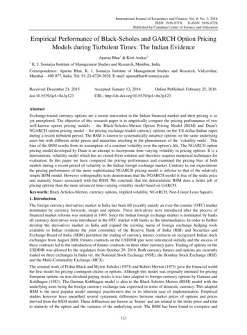
www.ccsenet.org/ijefInternational Journal of Economics and Finance𝑓(Ω) 𝑚𝑖𝑛𝜑 𝑛𝑖 1[𝐶𝑜𝑏𝑠,𝑖 (𝐾, 𝑇) 𝐶𝑀𝑜𝑑𝑒𝑙,𝑖 (𝑥1 , 𝑥2 𝑥𝑛 )]Vol. 8, No. 3; 20162(9)where Ω is the vector of parameter values to be determined by NLLS, 𝐶𝑜𝑏𝑠,𝑖 (𝐾, 𝑇) is the market price of the i thoption and 𝐶𝑀𝑜𝑑𝑒𝑙,𝑖 (𝑥1 , 𝑥2 𝑥𝑛 ) is the model price of the i th option. Calibrating the BSM is relatively simple asonly one parameter, i.e. the underlying volatility has to be estimated. We have used implied volatility backed outon the „t‟ day to price options on day „t 1‟ using the spot price, strike price, time to maturity and interest rates ofday t 1 thus giving us out-of-sample estimates of the option price.In the case of the GARCH model we have used the underlying exchange rate returns data as well as the optionsdata for calibrating the model as per a two-step procedure.We started with a five-year rolling window of daily exchange rate returns starting from May 1, 2008 ending withApril 30, 2013 and estimated the GARCH parameters 𝛼0 , 𝛼1 𝛼2 and θ* from this data using maximumlikelihood estimation (MLE). These initial parameters were used to estimate the conditional variance on the firstday of the month, i.e. May 2, 2013 and then Monte Carlo simulations were employed to simulate the optionprices on May 2, 2013 as per the GARCH option pricing model. The second step was to calibrate the originalMLE parameters to market prices using the NLLS technique. These new „implied‟ structural parameters wereused as initial parameters to simulate option prices for the subsequent day, i.e. May 3, 2013. Again theseparameters were calibrated to market option prices using NLLS. At the end of the month the initial five-yearwindow was rolled forward by deleting the earliest month and adding a new month. The structural parameters onthe first day of the new month were again estimated by MLE. This two-step procedure has been followed for theentire sample period. The calibrated „implied‟ parameters for each day have been used to determineone-day-ahead option prices based on the strike prices, interest rates and spot exchange rates of the next dayusing Monte Carlo simulation thus yielding out-of-sample estimates of the option price.We have used Excel VBA code (Chan & Wong, 2013) to perform the Monte Carlo simulations required forestimating the GARCH option model prices. Excel VBA has also been used to perform the minimization byopting for the GRG Nonlinear method and limiting the number of iterations to 1500. No restrictions were placedon the time taken for the iterations.5. Empirical Performance and ObservationsThis section documents the implied volatility pattern and the out-of-sample pricing performance of the models.Table 1 depicts the summary statistics of the daily USDINR returns over the period starting from May 1, 2008 toOctober 31, 2013. It is evident that the exchange rate returns data are negatively skewed and exhibit a largepositive kurtosis. The non-normality of the distribution is confirmed by the Jarque-Bera test statistic which is ahigh 954.34 with a p-value of zero.Table 1. Descriptive statistics of USDINR returns (May 1, 2013 to October 31, 2013)Descriptive MeasuresStatisticsDescriptive aProbability0.0062-0.02387.1527954.34000.0000The graph of the daily USDINR returns in figure 1 clearly reveals the time-varying nature of the volatility andvolatility clustering. An option pricing model based on an underlying GARCH process is therefore expected toperform better than the BSM which assumes normally distributed underlying data.128
www.ccsenet.org/ijefInternational Journal of Economics and FinanceVol. 8, No. 3; 2016Daily USDINR log 01250Figure 1. Daily USDINR returns (May 1, 2008-October 31, 2013)Table 2 depicts the descriptive statistics of the call option prices over the sample period. It can be seen thatnearly 84 per cent of the observations are short-term options and ATM calls make nearly 82 per cent of theobservations.Table 2. Descriptive statistics of the call option price (May 2013-October OTMAverageStd DevNumberAverageStd DevNumberAverageStd DevNumberAverageStd ITMDITMTotalTotal observations3872574177183156The pricing bias of the BSM model is well-documented in the literature. We have used the BSM to back out theimplied volatility from the market prices and analyzed the same within each moneyness-maturity bucket. Table 3summarizes the descriptive statistics of implied volatilities for different moneyness-maturity buckets.Table 3. Descriptive statistics of market implied volatility (May 2013-October OTMAverageStd DevAverageStd DevAverageStd DevAverageStd .06500.0059ATMITMDITMIt is evident from the table that implied volatilities vary systematically with respect to the strike prices over thesample period and make a smile pattern when they move from ATM options to OTM or DITM options. OTM,ITM and DITM calls exhibit the highest mean implied volatilities and ATM calls the lowest. Also average129
www.ccsenet.org/ijefInternational Journal of Economics and FinanceVol. 8, No. 3; 2016implied volatilities are seen to be highest for short-term options and tend to decline with increase in the maturityof the option. The standard deviation of implied volatilities is higher for short-term ITM and DITM options butdeclines for medium-term and long-term options.In accordance with existing research we have used three yard-sticks for measuring the empirical performance ofthe two models: (i) in-sample pricing errors (ii) out-of-sample pricing errors and (iii) Orthogonality tests. Thefollowing three error metrics have been employed to judge the pricing performance of the two models.1) Mean Absolute Percentage Error (MAPE).1𝑛 𝑛𝑖 1 𝐶𝑖,𝑚𝑜𝑑𝑒𝑙 𝑟𝑘𝑒𝑡 This is a measure of themagnitude of the pricing error.2) Mean Percentage Error (MPE)1𝑛 𝑛𝑖 1(𝐶𝑖,𝑚𝑜𝑑𝑒𝑙 𝐶𝑖,𝑚𝑎𝑟𝑘𝑒𝑡 ). This is a measure of the direction of the𝐶𝑖,𝑚𝑎𝑟𝑘𝑒𝑡pricing error.3) Mean Squared Error (MSE)1𝑛 𝑛𝑖 1(𝐶𝑖,𝑚𝑜𝑑𝑒𝑙 𝐶𝑖,𝑚𝑎𝑟𝑘𝑒𝑡 )2 . This is a measure of the volatility of thepricing error.5.1 In-Sample PerformanceIn-sample testing of the models reveals the consistency of the parameters with the option prices. Table 4 depictsthe mean and standard deviation for the parameter estimates for both
asset but with different strike prices and maturities resulting in the phenomenon of the „volatility smile‟. This bias of the BSM results from its assumption of a constant volatility over the option‟s life. The NGARCH option pricing model developed by Duan is an attempt to incorporate time-varying volatility in pricing options. It is a