WIXLIB

M. C. MODISETT, J. A. POWELLLocal volatility models generally employ a host of implied volatility parameters and few (if any) historicallyfitted variables. In contrast, stochastic volatility modelsemploy many historically-fitted parameters and only oneimplied parameter, the volatility. Jump process parameters are generally historically-fitted.As discussed above, current research tends to add newparameters to models in an effort to better reflect variousaspects of price movements. While doing this, one mustbe careful that new parameters not only improve the fitbut also that the degree of improvement warrants the newparameter. Below we will investigate a one-parameterextension of the BS model which accounts for a smallpricing drift. We evaluate its performance compared tothe original BS model from the perspective both of reflecting option prices and from that of parsimony: can theincreased complexity be justified statistically by the degree of improvement? We fit both the BS and our extension to S&P 500 Options data from 2003-2005; thetradeoff between additional complexity and improveddescription is assessed using the likelihood ratio test.2. Mathematical Model and MethodsHow would drift come about? There are two alternatives.On the one hand, it may be a small trend that market participants cannot observe. Actual calculations of the driftshow it to be quite small, small enough to not be detectable in a statistical analysis of price movements. Thisview of the drift is consistent with the contention thatmarket dynamics (alone) drive options prices, with negligible distortion by market participants. On the otherhand, the drift may be a trend perceived by market participants whether or not it actually exists in the market.This perceived drift alters market prices, but the necessary drift is not small enough to be discredited by statistical analyses. This view is consistent with the contentionthat market perceptions drive market prices, potentiallyindependent of actual price dynamics. Whichever interpretation appeals to the reader, the mathematics is thesame.It is interesting to note that this additional drift parameter may be viewed as arising from the assumptionthat the underlying security experiences periods of volatility and periods of relative stagnation. During volatileperiods, both random walk effects and interest rates impact option prices. However, during stagnant periods,any pricing effects due to volatility are dormant (by definition) but the interest rate clock would still be running.Thus the implied forward expectation from current option prices would conceptually be composed of twocomponents: one due to the volatility effect (with interestrates during volatile periods), and one due to interestrates (alone) during stagnant periods. The implied driftCopyright 2012 SciRes.599reflects the difference between interest rate effects andthe missing random walk effects over the stagnant periods. The implied drift effect could be positive or negativesince the stochastic process during active periods (implied by volatility) could create a forward expectancyabove or below that implied by interest rates.2.1. Deriving an Extension of the Black-ScholesModelThe traditional derivation of BS begins by consideringthe neutral hedge equity constructed by selling a ratio 1 w of call option in a stock per share of stock held. x Consider the stock and hedging options as a separateportfolio. For such a portfolio the net equity (E) investedis w E x N ,wx where N is the number of shares of stock held, and subscript notation for partial derivatives is adopted (that is,wx x w ). Thus E N x wx 1 w ,is the net change in portfolio value with changes in eitherstock or option price. Applying the usual arbitrage-freeargument originally introduced by Black, Merton andScholes, it is required that option prices evolve over timeso that equity value experiences growth according torisk-free interest rates. This is natural since the combination of stocks and hedging options constitutes a risk-freeportfolio. Mathematically, E N x wx 1 w N x wx 1 w r t ,(2)where r is the risk-free interest rate. Option price is expected to vary with both time and price of underlyingstock; using Taylor’s theorem changes in option pricemay be replaced with related changes in stock price intime,1 w wx x wxx x 2 wt t2 (3) O t , x t , x .23The next step would be to substitute (3) into (2) andthereby derive a differential equation for option prices.However, to consistently neglect terms of differing orderas t 0 , there must be an assumption about howchanges in stock price, x, vary with changes in time.As done in the traditional BS assumption, here the assumption is that stock prices follow a random walk process with standard deviation vx in which the market volatility is v. Departing from BS, however, the random walkAM

M. C. MODISETT, J. A. POWELL600is assumed to have a slight bias (as opposed to zeromean). Thus are made the following assumptions aboutthe expectation, , of quantities in (2) and (3): x cx t ,. reflecting the (small) bias, or drift, in ran-dom steps,(4a)wx x 0, reflecting market participants’ inability toperceive bias in the underlying carries over to an inabilityto perceive bias in the option price,(4b) x 2 v 2 x 2 t , reflecting growth of variance in therandom walk.(4c)Here the parameter c may be positive or negative andreflects the expected drift or trend of underlying stockprices. Note that for this to be a consistent approximationit is required that c O v ,2meaning that the drift parameter will be small in comparison to volatility, since v 1 (which dovetails withthe assumption that it is too small for market makers totake into consideration).Multiplying (2) by wx, canceling a common factor of N,substituting (3) into (2), replacing the various changes instock price with their expectations in (4), dividing by tand taking the limit t 0 leads directly to: w w1 2w r c x rw v 2 x 2 2 , t x2 xwith u z, 0 S max e z 1, 0 .Changing to a traveling frame of reference1 z c r v 2 to remove the lowest order z2 derivative gives a simple diffusion equation:u 1 2v u ,2with u , 0 S max e 1, 0 .The convolution form of the general solution for thediffusion equation is u , 2πv 2 1 2 f y exp 2yv dy, 22 where f is the initial condition. Applying this formof the solution to the initial conditions above, and notingthat the integrand will be zero for y gives u , 2πv 2 1 2 S e y y2 1 exp 2 2v dy. From here, completing the square and usingerf z (5)2z eπ t 2dt0where c is the implied drift parameter. This is the Extended Black-Scholes (EBS) model. BS’s differentialequation can be recovered by setting c to zero. Note thatthis drift measures the deviation not from current prices,but rather deviation from the interest rate applied to current prices (the arbitrage-free estimate of future pricesrelative to current prices).gives2.2. Solution of the Extended Black-ScholesEquationReturning to the original coordinates, simplifying,evaluating at t 0 and employing the identity1 z z 1 erf , where Ф is the standard nor2 2 We seek to solve (5) with a boundary condition at maturity (t t*) given by w x, t t max x S , 0 .u , x is introduced to remove the non-constant coefficients andexponential growth term, as well as to translate the condition at maturity into an initial condition, givingu 1 21 v u zz c r v 2 u z ,22 Copyright 2012 SciRes.2 12 v 2 e 1 erf 1 erf 2 2v v 2 2v 2 2 . mal cumulative distribution function, givesw xe ct d Se rt d , Introducing a change of variables, t t , z ln , w e r u z, ,S (6)where1 x ln r c v 2 t 2 S.d 2 vtUnder the assumption that c 0 this reduces to theoriginal BS option pricing formula.AM

M. C. MODISETT, J. A. POWELL3. Data Analysis and Model CompetitionIn the absence of a market trend (c 0), with x, r, S andt* assumed known, (6) gives a one-to-one relationshipbetween volatility and option price. Inverting this relationship individually for a series of options, differingonly in strike price, often gives a non-constant volatility(the “smile” or “smirk”). However, when c is not zero,how should one proceed? A direct analog to the aboveprocedure would require selecting pairs of options sharing all parameters save strike price, then solving the resulting nonlinear system of equations for v and c. Butwhich pairs should be selected? Or if all possibly pairsare considered, how are results to be interpreted? Are thedifferences significant? This latter question, in fact, applies also to the volatility smile: given the backgroundvariability in underlying stock prices and volatility, arethe differences among applied volatilities really significant?In this paper, an alternate approach is employed following a model competition and selection perspectiveadvanced by Hilborn and Mangel in 1997 [18]. In thisapproach, model parameters for competing models are fitto all available data using maximum likelihood, cognizant of the fact that there is process variability in the witnessed parameters (e.g. stock prices are clearly not fixedthrough the course of a day) as well as observationalvariability (e.g. different market participants may assessvolatility using different metrics, over different periodsof time, yielding different option prices). Model parameters are chosen to maximize likelihood, and the modelwhich accounts for the most variability among alternativemodels, with maximum parsimony, should be considered“best”.3.1. Statistical MethodsThe EBS vis-à-vis the BS constitutes a case of nestedmodels, in which the simpler model is realized by a particular choice of parameters in the more complex. A likelihood ratio test may be used to characterize the signifycance of differences between nested models. Assumingboth models are fit to data using maximum likelihood,the statisticR 2 L data model1 L data model2 ,is distributed according to a chi-squared distribution withnumber of degrees of freedom equal to the difference innumbers of parameters between model 1 (the simpler)and model 2 (the more complex, in which model 1 isnested). HereL data model j 11ln 2π e2 222 e w j wobs 2datais the negative log-likelihood of model j given the obCopyright 2012 SciRes.601served data, with wj being the model prediction for themaximum likelihood parameters, wobs being the observedoption price and e being the standard deviation of theerrors (see [18] for details). Because the difference inthese logs is the log of the ratio of the likelihoods, thistest is called the likelihood ratio test. The resulting chisquared probability can be viewed as the probability thatthe more complex model is an improvement over thesimpler nested model (that is, the probability that thesimpler model’s parameters lie outside the correspondingparametric confidence interval of the more complexmodel). General wisdom states that parameters shouldnot be added without penalty; the above procedure penalizes the more complex model for its higher number ofparameters via the numerical degrees of freedom in thechi-squared distribution.To determine c and v for each day of data in our EBSmodel and v for the BS model, we minimize the negativelog likelihoods of each over the strike prices for that day.Furthermore, the negative log likelihood of each model isused in the likelihood ratio test, as described above. Acorresponding p value was determined from the chisquared distribution with one degree of freedom, indicating the probability that the more complex model (EBS)is a significant improvement over its simpler companion(BS) for that day.3.2. DataWe use data from the Option Price Reporting Authority(OPRA) for S&P 500 index calls maturing December(19), 2006. The data runs from November 5, 2003 toNovember 3, 2005. Option Price Reporting Authorityprovides consolidated option information and is a committee administered jointly by the five option exchanges:AMEX, BOX, CBOE, CBOT, ISE, PCX, PHLX. Ourdata came indirectly through a third-party vendor. Weexcluded 5 dates in which the data seemed in error: forthe 1325 strike in 2003, November 20, 21, 25, and December 8, 16 and 22; for the 1125 strike, the prices in2005 of October 24, 25 and 28 and November 2 alsoseemed probably in error. In the 1150 Strike, the following dates are excluded: 2005 October 19, 24, November3. We consider only contracts whose strike is between1125 and 1375, inclusive, and which is a multiple of 25.This has the effect of concentrating on contracts morelikely to be liquid and traded, and to eliminate sporadicor illiquid contracts. During this time:1) The S&P 500 index grew from 1051.81 to 1219.94,with a minimum of 1033.65 (November 20, 2003) and amaximum of 1245.04 (August 3, 2005). The True Range(daily high minus daily low) expressed as a percent ofthe index value varied from 0.25% to 2.14%, with anaverage of 0.91% and a standard deviation of 0.37%.AM

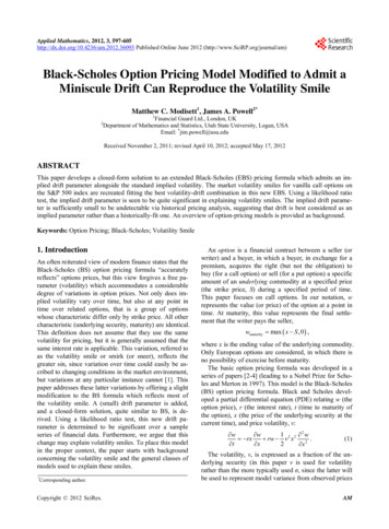
602M. C. MODISETT, J. A. POWELL(See Figure 2).2) Average transaction volume per contact grew fromabout 332 contracts (averaged over 5 working days) topeak of 3476 and ending at 2003 contracts (See Figure3). This increase is a natural consequence of comingcloser to maturity since the shortest dated options are themost traded and liquid.3) Excluding the 1125 strike contract and certain daysdue to data issues, implied volatilities varied from 7.57%to 16.05%, with an average of 10.94% and a standarddeviation of 1.23%. For each day, the difference betweenmax and min implied volatilities (for days in which morethan one contract was traded, and excluding 1125 and1150 strikes) varied from 0.26% to 6.43%, averaging1.92% with a standard deviation of 1.04%.4) We note that the closing price for each option andthe index were used. This is a potential source of inconsistency since the last trade for an option contract maynot occur at the end of the last moment of stock trading(applicable for the index). Our model, like BS, assumesthat the current price of the index is used. Option exchanges generally close before stock exchanges, so closing option and index prices seldom occur simultaneously.Even if the data from within a day were used to synchronize option and index prices, the result may not be asmarket participants view the market. Market makers mayFigure 2. S&P 500 index. The underlying commodity behavior for the options considered, over the time period November 2003 to November 2005.Figure 3. Daily option volume. For each day, the averagevolume for option contracts in the series studied. As optioncontracts approach maturity, volume naturally increasessince most trading is done in the nearest contract.Copyright 2012 SciRes.well have a backlog of orders in either the option or theshares, such that a market maker could reliably see thatthe price will move in one direction. Thus the marketmaker would use an index price in the option formulathat differs from the current index price.3.3. Analysis of Data: ResultsTo compare the EBS model to the no-drift BS, two fittings are performed. First each day’s closing optionprices are fit in the BS to the best implied volatility (onevolatility for all options) that maximizes the likelihood ofthe model given actual option prices. Second, for eachday, the EBS is fit for the best combination of drift andimplied volatility (one combination for all options on thatday) maximizing the likelihood.To evaluate the results on each day, the worst and average per-day price difference between actual and modelare chosen. The error is considered as a percent of theunderlying closing index price on that day, with the results summarized in Table 1. The error is approximatelyhalved by the addition of an implied drift parameter. Thisis true whether looking at the worst price of each day, orthe average over all option prices. The ratio of standarddeviation to average for the error term does not changesignificantly when adding a drift parameter.Using a likelihood ratio test for each day, the drift parameter is seen to have over a 95% chance of improvingfit in 297 out of 344 days. Insight can be gained by comparing this statistic with the implied drift for each corresponding day. Figure 4 illustrates that the low chances ofimproving the model occur on those days in which driftvalues are close to zero. This is to be expected, given thatthe probability of improvement depends on where thesingle parameter BS volatility estimate falls relative tothe confidence interval for the drift volatility estimatefor EBS. The EBS fails to be clearly better exactly whereits parameters become indistinguishable from the no-driftTable 1. Comparison of residuals, Classic BS with andwithout drift. The modified BS model with drift (called EBS)significantly reduces variability of volatility estimates overthe classical BS model. The average variation in each day isgenerally halved, while the worst fit for each day (an outlier)is also reduced. Further reduction in variability may not bemeaningful.Classic BS(No drift)EBS(With drift)Max Error over Period0.87%0.58%Average Error (Each Day’s Worst)0.27%0.13%Average Error (All Prices)0.15%0.07%Std. Dev. of Error (Each Day’s Worst)0.14%0.09%Std. Dev. of Error (All Prices)0.11%0.06%AM

M. C. MODISETT, J. A. POWELLFigure 4. Probability that EBS improves BS. Most often, thechance is 100% that EBS improves BS. The lower probability cases correspond to when the drift is close to zero andthe two models are less distinguishable.BS. This supports the contention that the implied driftparameter significantly improves the model’s fit to actualprices overall.603Figure 5. Comparison of implied volatility estimates fromEBS and BS. The EBS model’s implied volatility estimate isgenerally less than that of BS, but the two track each otherreasonable well.4. DiscussionThe EBS model makes a significant improvement, butperhaps adding more parameters could provide additionalsignificant increases in fit. To the knowledge of the authors, there is no mathematical or statistical method fordetermining whether or not further parameters could bejustified. Rather, practitioners need to look at the dataand its context to determine whether or not additionalparameters could be warranted. Here it is argued that thecloseness of fit using implied volatility-drift in the EBSprobably is as close as the data could reasonably allow.Referring back to Table 1, the average price error foran option in the new model is 0.07%, and the averageworst for each day is 0.0013%. Can we expect greater fitthan this? These price variations are similar to bid-askspreads on many illiquid securities. Options have nowhere near the liquidity enjoyed by the underlying index.To attempt any greater fitting of option prices would demand explanations of variations with a magnitude similarto that of bid-ask spreads in the security. This wouldseem unreasonable for a pricing model that ignores suchbid-ask spreads. The conclusion is that the fit offered bythe EBS may be as close as is reasonable.When introducing implied parameters into a model,one should observe how the parameter evolves over timeto ensure that the implied parameter is neither too stablenor too erratic. If too stable, the implied parameterprobably masks another effect more appropriate for direct modeling. Figure 5 compares the evolution of theimplied volatilities that arise from the no-drift (BS) andwith-drift (EBS) cases. (Gaps are due to removed datapoints.) The two volatilities track each other, with theno-drift volatility being higher than the other in practically all cases.Figures 6 and 7 depict the evolution of the implieddrift parameter. Figure 6 displays the parameter itselfexpressed as a rate similar to interest rates. This is the cCopyright 2012 SciRes.Figure 6. Implied drift in the EBS model (expressed as arate). The above annualized rates are generally small—thedaily price movement would be below what could be detected with statistical studies. The drift parameter becomeserratic closer to maturity as a consequence of annualizingrate on a short-term instrument; this effect is accounted forin the next figure.Figure 7. Implied drift in the EBS model (expressed as adiscount price). Estimated drift rate data is converted toprice data. The implied drift parameter evolves well, neither staying too static nor too fl

Keywords: Option Pricing; Black-Scholes; Volatility Smile . 1. Introduction . An often reiterated view of modern finance states that the Black-Scholes (BS) option pricing formula "accurately reflects" options prices, but this view forgives a free pa- rameter (volatility) which accommodates a considerable degree of variations in option prices.