WIXLIB

8take either call or put- giving us total 8 single barrier types. Barriers also come invarious other forms including double barriers, parisians, and partial time barriers.Here, our discussion only target on single barrier types.2.1Valuation MethodsThe valuation of barrier options can be tricky, because unlike other simpler options they are path-dependent — that is, the value of the option at any timedepends not just on the underlying at that point, but also on the path taken bythe underlying since if the barrier is crossed the option is initiated or exterminated. Although the classical Black–Scholes approach does not directly apply, severalmore complex methods can be used.An approach is to study the law of the maximum (or minimum) of the underlying. This approach gives explicit prices to barrier options under the Black-Scholesframework. Also when an exact formula is difficult to obtain, barrier options canbe priced with the Monte Carlo path simulation. However, computing the Greeks(sensitivities) using this approach is numerically unstable.2.2Analytical Solution under the Black-Scholes ModelUsing the methods of equivalent martingale pricing (risk neutral valuation principle), the price of a down-and-out put barrier option at time zero with respect tomaturity T , strike K, barrier Sb , initial stock price S is given by:Pdop (ST , K, Sb) e rT E Q [(K ST )1{K ST ,mT0 Sb } ](2.1)

9Note:1. The realized minimum value of underlying stock from time zero to time t isdefined as mt0 min Su .0 u t2. The indicator function 1A (X) where:1A (X) 1 ifX A 0 otherwiseis a useful notational device, in probability theory: if X is a probability spacewith probability measure P and A is a measurable set, then 1A becomes arandom variable whose expected value is equal to the probability of A:E(1A ) ZX1A (x)dP ZAdP P (A)(2.2)In view of linearity of the expectation, the above equation of down-and-out putoption price Pdop (ST , K, Sb) can break into four terms:Pdop (ST , K, Sb) e rT (E Q [(K ST )1{ST K}] E[(K ST )1{ST Sb } ] E[(K ST )1{ST Sb ;mT0 Sb } ] E[(K ST )1{ST K;mT0 Sb } ])(2.3)In the above equation, the first term is the price of a vanilla European put optionunder the Black-Scholes model.

10The second term is similar to the Black Scholes put price.e rT E Q [(K ST )1{ST Sb } ] Φ( d2 (Sb ))Ke rT Φ( d1 (Sb ))S0(2.4)2ln SSbt (r σ2 )(T t) d1,2 (Sb ) σ T tThe value of the last two terms in price function Pdop (ST , K, Sb ) requires thedetermination of the joint distribution function of ST and mT0 . Therefore, weapply the following theorems to solve the problem. Theorem 1 (Reflection Principle)Let Wt0 denote the Brownian motion that starts at zero, with constant volatility σ and zero drift rate. ξ inf{t : Wt0 h}.Ŵt0 Wt0 ,t ξ 2h Wt0 ,ξ t TThen Ŵt0 is also a standard Brownian motion. Theorem 2 (Girsanov’s Theorem)Girsanov’s Theorem begin with a Brownian motion under measure P andthen construct a new measure Q under which a “translated” process is aBrownian motion.So assume that {WtP }t 0 defined on (Ω, F, P) is a Brownian motion startingfrom zero. Now define for an process {γs }s 0 adapted to the filtration {Ft }t 0RtZt e0γs dWsP 12Rt0γs2 ds(2.5)

11E[Zt ] 1 and for each T 0 define a new probability measure Q on {Ft }t 0byQ E(1A ZT ) f or A FTDefine a process WtQ WtP Rt0(2.6)γs ds. Then for each fixed T the processWtQ is a Brownian motion on (Ω, FT , Q)We illustrate how the reflection principle is applied to derive the joint law of theminimum value over [0,T ] and terminal value of a Brownian motion. Regardingto pricing a barrier option, we would like to find P (Wtu k, mt0 h) To figureout the last two terms, we construct three transformation equations to apply thereflection principle and the Girsanov’s Theorem.r 21 σ 2g σSb1h ln( )σS01Sbk ln( )σS0(2.7)(2.8)(2.9)

12To calculate the last term of (2.4):e rT E Q [(K ST )1{ST K;mT0 Sb } ] e rT (KE Q [egWT 2 g T 1{W Q k;Q1 2T E Q [egWT 2 g T S0 eσWT 1{W Q k;QQ1 2Tinf WtQ h} ]0 t Tinf WtQ h} ])0 t T e rT (Ke 2 g T E Q [e{g(2h WT )} 1{2h W Q k;Q1 2T e 2 g T E Q [(e{(g σ)(2h WT )} 1{2h W Q k;Q1 2T1 2T 2hg e rT (Ke 2 g 21 g 2 T 2h(g σ) einf WtQ h} ]0 t Tinf WtQ h} ])0 t TE Q [e{ gWT )} 1{2h W Q k} ]QT{(g σ)( WTQ )}E Q [(e1{2h WTQ k} ])(2h k) (g σ)T )]σ T1 2(2h k) (g σ)T S0 e2h(g σ) gσT 2 σ T Φ()σ T e rT [Ke2hg Φ(Now we can re-plug in g, h, k, thus get the expression of the last term of (2.4)Then we put all derivations into a formula that represents Pdop to be the value of this down-and-out put barrier option:pdop (S0 , K, Sb) Ke rT Φ( d2 ) S0 Φ( d1 ) S0 Φ( x1 ) Sb Ke rT Φ( x1 σ T ) S0 ( )2η [Φ(y) Φ(y1 )]S0 Sb Ke rt ( )2η 2 [Φ(y σ T ) Φ(y1 σ T )]S0with2S ln( S0bK )r 21 σ 2 η ησ,y T,σ2σ T ln( SS0b )ln( SS0b )x1 ησ T , y1 ησ Tσ Tσ T(2.10)

13This analytical solution for continuously monitored down-and-out put barrier option is also in accordance with the formula given in [13]:Pdop (So , K, Sb) S0 e rT (Φ(d3 ) Φ(d1 ) b[Φ(d8 ) Φ(d6 )]) Ke rT (Φ(d4 ) N(d2 ) a[Φ(d7 ) Φ(d5 )])withSb 1 2r2σ)S02rSbb ( )1 σ2S0ln SK0 (r 12 σ 2 )T d1 σ Tln SK0 (r 21 σ 2 )T d2 σ Tln SS0b (r 21 σ 2 )T d3 σ Tln SS0b (r 21 σ 2 )T d4 σ Tln SS0b (r 21 σ 2 )T d5 σ Tln SS0b (r 21 σ 2 )T d6 σ Tln SS0 2K (r 21 σ 2 )Tb d7 σ T1 2ln SS0 K2 (r 2 σ )Tb d8 σ Ta ((2.11)

142.2.1A Continuity Correction to Discrete Barrier OptionThe barrier option pricing formulas presented so far assume continuous monitoring of the barrier. In practice, the barrier is normally monitored only at discretepoints in time. An exception is the currency options market, where the barrieris frequently monitored almost continuously. For equity option in our case, thebarrier is typically monitored against an periodical time point price. Discretemonitoring will naturally lower the probability of barrier hits compared with continuous barrier monitoring. Broadie, Glasserman and Kou [7] showed theoreticallyand through examples that discrete barrier options can be priced with remarkableaccuracy using the following simple correction.Sb is the continuous barrier options formulas with a discrete barrier level Sd equal toSd Sb eβσ tif the barrier is above the underlying security, and toSd Sb e βσ tif the barrier is below the underlying security. At is the time between monitoringevens, and β 0.5826.

152.3Monte Carlo MethodsMonte Carlo methods are based on the analogy between probability and volume.The mathematics of measure formalizes the intuitive notion of probability, associating an event with a set of outcomes and defining the probability of the eventto be its volume or measure relative to that of a universe of possible outcomes.Monte Carlo uses this identity in reverse, calculating the volume of a set by interpreting the volume as a probability. In the simplest case, this means samplingrandomly from a universe of possible outcomes and taking the fraction of randomdraws that fall in a given set as an estimate of the set’s volume. The law of largenumbers ensures that this estimate converges to the correct value as the number ofdraws increases. The central limit theorem provides information about the likelymagnitude of the error in the estimate after a finite number of draws.In mathematical finance, a Monte Carlo option model uses Monte Carlo methods to calculate the value of an option with multiple sources of uncertainty orwith complicated features.The term ‘Monte Carlo method’ was coined by Stanislaw Ulam in the 1940s.The first application to option pricing was by Phelim Boyle in 1977 (for Europeanoptions). In 1996, M. Broadie and P. Glasserman showed how to price Asian options by Monte Carlo. In 2001 F. A. Longstaff and E. S. Schwartz developed apractical Monte Carlo method for pricing American-style options.We look at a simple example of European call option. Consider the option granting the holder the right to buy the stock at a fixed price K at a fixed time T in

16the future; the current time is t 0. The payoff to option holder is(ST K) max[0, ST K](2.12)To get the present value of this payoff we multiply by a discount factor e rT . Wedenote the expected present value by E[e rT (ST K) ]As we know we apply the risk neutral measure into the calculation of the aboveexpectation. The solution to the Black-Scholes SDE dSt /St rdt σdWt Q underrisk neutral measure is1ST S0 e[(r 2 σ2 )T σWT](2.13)The random variable WT is normally distributed with mean 0 and variance T . Wemay therefore represent the terminal stock price as1ST S0 e[(r 2 σ2 )T σ T Z](2.14)where Z is a standard normal variable.Then we can simulate the path of stock price and apply the Monte Carlo samplingmethods to estimate price of the option by the expectation form E[e rT (ST K) ] .2.3.1The Main Framework of Monte CarloSuppose we want to estimate some quantity θ E[h(X)], where X {X1 , X2 , ., Xn }is a random vector in Rn . h(·) is a function from Rn to R, and E[ h(X) ] .Note that X could represent the values of a stochastic process at different pointsin time. For example, Xi might be the price of a particular stock at time i and

17h(·) might be given by:h(X) X1 X2 . Xnn(2.15)so then θ is the expected average value of the stock price. To estimate θ we usethe following algorithm:Monte Carlo Algorithmfor i 1 to ngenerate Xiset hi h(Xi )bset θn h1 h2 . hnnThere are two reasons which show why θb to be a good estimator:1. θbn is an unbiased estimator.E[θbn ] Pni 1nhi Pnnθh(Xi ) θnni 12. θbn is consistent. That is:θbn θ with probability 1 as n (2.16)(2.17)This is followed by Strong Law of Large Numbers.Note that we can also estimate probabilities this way by representing them asexpectations. In particular, if θ P(X A), then θ E[1A (X)].We consider simple forms of barrier options. A down-and-out European put op-

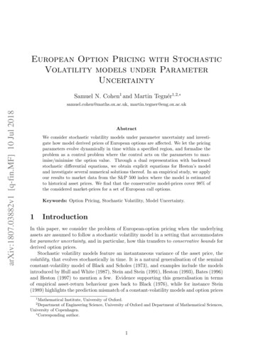
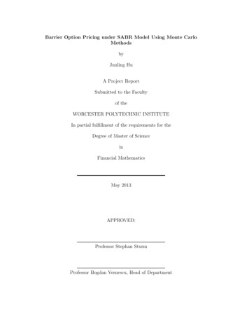
18tion.Its payoff at the expiry is given by the product:1{K ST ,mT0 H} · (K ST ) (2.18)The risk-neutral price of the down-and-out European call option at time 0 is theexpected discounted payoffPdop E[1{K ST ,mT0 H} (K ST ) ]2.3.2(2.19)Variance Reduction TechniquesWe have seen in last section that one way to improve the accuracy of an estimateis to increase the number of replications n, since Var(X̄(n)) Var(Xi )/n. However, this brute-force approach may require an excessive computational effort. Analternative is to work on the numerator of this fraction and to reduce the varianceof the samples Xi directly. This may be accomplished in different ways, more orless complicated, and more or less rewarding as well. [14]Antithetic samplingSuppose as usual that we would like to estimate θ E[h(X)] E[Y ], and that wehave generated two samples, Y1 and Y2 . Then an unbiased estimate of θ is givenbyY1 Y2θb 2(2.20)

19andb Var(θ)Var(Y1 ) VarY2 2Cov(Y1 , Y2 )4(2.21)In the antithetic path plot example: we construct the estimator by using twoAntithetic Sampling22.822.6Stock Price22.422.22221.8Primary PathAntithetic Path21.600.010.020.030.04Time (Years)0.050.060.07Figure 2.1: Antithetic Path ExampleBrownian motion trajectories that are mirror images of each other. This causescancellation of dispersion.b If Y1 and Y2 are IID, then Var(θ)Var(Y ).2bHowever, we could reduce Var(θ)if we could arrange it so that Cov(Y1 , Y2 ) 0. We now describe the method of antithetic variates for doing this. We will begin with the case where Y is a functionof IID U(0, 1) random variables so thatθ E[h(U)]

20where U (U1 , ., Um ) and the Ui ’s are IID U(0, 1). The crude Monte Carloalgorithm, assuming we use 2n samples, is as follows: In the above algorithm,Crude Simulation Algorithm for Estimating θfor i 1 to 2ngenerate Uiset Yi h(Ui )end forP2nset θb2n Ȳ2n i 1 Yi /2nP2n2set σb2n i 1 (Yi Ȳ2n )2 /2n 1σb2nset approx. 100(1 α)% CI θb2n z1 α/2 2nhowever, we could also used the 1 Ui ’s to generate sample Y values, since ifUi U(0, 1), then so too is 1 Ui . We can use this fact to construct another(i)(i)estimator θ as follows. As before, we set Yi h(Ui ), where Ui (U1 , ., Um ).(i)(i)We now also set Ỹi h(1 Ui ), where we use 1 Ui to denote (1 U1 , ., 1 Um ).Note that E[Yi ] E[Ỹi ] so that in particular, ifZi : Yi Ỹi,2then E[Zi ] θ. This means that Zt is an also unbiased estimator of θ. If theUi ’s are IID, then so too are the Zi ’s and we can use them as usual to computeapproximate confidence interval for θ. We say that Ui and 1 Ui are antitheticvariates and we then have the following antithetic variate simulation algorithm.As usual, θba,n is an unbiased estimator of θ and the Strong Law of Large Num-bers implies that θba,n θ almost surely as n . Each of the two algorithmswe have described above uses 2n samples so the question naturally arises as towhich algorithm is better. Note that both algorithms require approximately thesame amount of effort so that comparing the two algorithms amounts to comput-

21Antithetic Variate Simulation Algorithm for Estimating θfor i 1 to ngenerate Uiset Yi h(Ui ) and Ỹi h(1 Ui )set Zi (Yi Ỹi )/2end forPset θbn,a Z n ni 1 Zi /nPn2set σbn,a i 1 (Zi Z n )2 /n 1σbset approx. 100(1 α)% CI θba,n z1 α/2 n,aning which estimator has a smaller variance.It is easy to see thatandVar(θb2n ) Var(PnP2ni 12nZiYi) Var(Y )2nVar(Z)nnbVar(Y Y )Var(Y ) Cov(Y, Yb ) 4n2n2nbCov(Y, Y ) Var(θb2n ) 2nVar(θbn,a ) Var(i 1) Therefore, Var(θbn,a ) Var(θb2n ) if and only if Cov(Y, Yb ) 0Control VariateSuppose again that we wish to estimate θ : E[Y ] where Y h(X) is the outputof a simulation experiment. Suppose that Z is also an output of the simulation or

22that we can easily output it if we wish. Finally, we assume that we know E[Z].Then we can construct many unbiased estimation of θ:1. θb Y , our estimator2. θbc Y c(Z E[Z])where c is some real number. It is clear that E[θbc ] θ. The question is whether orb To answer this question, we compute Var(θbc )not θbc has a lower variance than θ.and obtainVar(θbc ) Var(Y ) c2 Var(Z) 2c Cov(Y, Z)(2.22)Since we are free to choose c, we should choose it to minimize Var(θbc ). Simplecalculus then implies that the optimal value of c is given byc Cov(Y, Z)Var(Z)(2.23)Substituting for c in () we see thatCov(Y, Z)2Var(Z)2b Cov(Y, Z) Var(θ)Var(Z)Var(θbc ) Var(Y ) So we see that in order to achieve a variance reduction it is only necessary thatCov(Y, Z) 6 0. In this case, Z is called a control variate for Y . To use the controlvariate Z in our simulation, we would like to modify our algorithm so that aftergenerating n samples of Y and Z we would simply setθbc Pni 1 (Yi c (Zi E[Z]))n(2.24)

23Control Variate Simulation Algorithm for Estimating θ/*Do pilot simulation first*/for i 1 to pgenerate (Yi , Zi )end forcompute bc /*Now do main simulation*/for i 1 to ngenerate (Yi , Zi )set Vi Yi bc (Zi E[Z])end forPnset θbbc V n i 1 Vi /nPn(Vi θbbc )2 /n 1set σb2 n,vi 1σbset approx. 100(1 α)%CI θbbc z1 α/2 n,vnThere is a problem with this, however, as we usually do not know Cov(Y, Z). Weovercome this problem by doing p pilot simulation and settingdCov(Y,Z) Ppj 1 (Yi Y p )(Zj E[Z])p 1If it is also the case that Var(Z) is unknown, then we also estimate it withand finally setdVar(Z) Ppbc j 1(Zj E[Z])2p 1dCov(Y,Z)dVar(Z)Assuming we can find a control variate, our control variate simulation algorithm isas follows. Note that the Vi ’s are IID, so we can compute approximate confidenceinterval as before.

24Conditional Monte CarloWe now consider the conditional Monte Carlo variance reduction technique. Theidea here is very simple. As was the case with control variates, we use our knowledge about the system being studied to reduce the variance of our estimator. Asusual, suppose we wish to estimate θ E[h(X)] where X (X1 , ., Xm ). Ifwe could compute θ analytically, then this would be equivalent to solving an mdimensional integral. However, maybe it is possible to evaluate part of the integralanalytically. If so, then we might be able to use simulation to estimate the otherpart and thereby obtain a variance reduction.Let X and Z be random vectors, and let Y h(X) be a random variable. Supposewe setV E[Y Z](2.25)Then V is itself a random variable that depends on Z, so that we may writeV g(Z) for some function, g(·). We also know thatE[V ] E[E[Y Z]] E[Y ](2.26)so that if we are trying to estimate θ E[Y ], one possibility would be to simulateV’s instead of simulating Y’s. In order to decide which would be a better estimatorof θ, it is necessary to compare the variances of Y and E[Y Z]. To do this, usingthe conditional variance formula:Var(Y ) E[Var(Y Z)] Var(E[Y Z])Now Var(Y Z) is also a random variable that depends on Z, and since a varianceis always non-negative, it must follow that E[Var(Y Z)] 0. But then impliesVar(Y ) Var(E[Y Z])

25so we can conclude that V is a better estimator of θ than Y.To see this from another perspective, suppose that to estimate θ we first haveto simulate Z and then simulate Y given Z. If we can compute E[Y Z] exactly,then we can eliminate the additional noise that comes from simulating Y given Z,thereby obtaining a variance reduction. Finally, we point out that in order for theconditional expectation method to be worthwhile, it must be the case that Y andZ are dependent.We want to estimate θ : E[h(X)] E[Y ] using conditional Monte Carlo. Todo so, we must have another variable or vector, Z, that satisfies the followingrequirements: 1. Z can be easily simulated 2. V : g(Z) : E[Y Z]can be computed ex

1.3 Summary of Vanilla Option Pricing under the Black Scholes To price the option, we denote the value of the option C, on an underlying asset St which pays a function f(ST) at maturity time T. The interest rate, which is constant, to be r. The payoff at maturity of an European call option with strike price K is defined by f(ST) max(ST .