Transcription
Woraphon WATTANATORN, Kedwadee SOMBULTAWEE /Journal of Asian Finance, Economics and Business Vol 8 No 2 (2021) 0685–0695685Print ISSN: 2288-4637 / Online ISSN 2288-4645doi:10.13106/jafeb.2021.vol8.no2.0685The Stochastic Volatility Option Pricing Model: Evidence from a HighlyVolatile MarketWoraphon WATTANATORN1, Kedwadee SOMBULTAWEE2Received: November 05, 2020Revised: January 05, 2021 Accepted: January 15, 2021AbstractThis study explores the impact of stochastic volatility in option pricing. To be more specific, we compare the option pricing performancebetween stochastic volatility option pricing model, namely, Heston option pricing model and standard Black-Scholes option pricing. Ourfinding, based on the market price of SET50 index option between May 2011 and September 2020, demonstrates stochastic volatility ofunderlying asset return for all level of moneyness. We find that both deep in the money and deep out of the money option exhibit highervolatility comparing with out of the money, at the money, and in the money option. Hence, our finding confirms the existence of volatilitysmile in Thai option markets. Further, based on calibration technique, the Heston option pricing model generates smaller pricing error forall level of moneyness and time to expiration than standard Black-Scholes option pricing model, though both Heston and Black-Scholesgenerate large pricing error for deep-in-the-money option and option that is far from expiration. Moreover, Heston option pricing modeldemonstrates a better pricing accuracy for call option than put option for all level and time to expiration. In sum, our finding supports theoutperformance of the Heston option pricing model over standard Black-Scholes option pricing model.Keywords: Stochastic Volatility, Option Pricing Models, Performance Comparison, Heston Option Pricing Model, Nonconstant VolatilityJEL Classification Code: G10, G11, G131. IntroductionIn 1973, Black and Scholes developed a model to pricecontingent claim named Black-Scholes option pricing model(Black & Scholes, 1973). This option pricing is well knownamong both academicians and practitioners due to an easinessto use. As a consequence, the Black-Scholes (BS) model isuseful and convenient to value option price for both portfoliomanagement and risk management purposes. However, dueFirst Author and Corresponding Author. Lecturer in Finance,Department of Finance, Thammasat Business School, ThammasatUniversity, Thailand [Postal Address: 2 Phra Chan Road,Phra-Borom Maha-Ratchawang, Phra-Nakhon, Bangkok 10200,Thailand] Email: woraphon@tbs.tu.ac.th2 Assistant Professor in Marketing, Department of Marketing,Thammasat Business School, Thammasat University, Thailand.Email: kedwadee@tbs.tu.ac.th1 Copyright: The Author(s)This is an Open Access article distributed under the terms of the Creative Commons AttributionNon-Commercial License (https://creativecommons.org/licenses/by-nc/4.0/) which permitsunrestricted non-commercial use, distribution, and reproduction in any medium, provided theoriginal work is properly cited.to its reliance on strict assumptions, the BS model assumesthat underlying asset prices follow a geometric Brownianmotion (GBM) process with known, and constant of meanand variance. Besides, BS assumes a constant risk-freerate, no transaction costs, and continuous trading. Basedon mentioned unrealistic assumptions for the real world,the pricing accuracy of the BS model is questionable. Further,many empirical studies report that the BS hardly predictsoption price correctly, principally because its assumptionof constant volatility is incorrect. Volatility is not constant;it moves stochastically over time (Geske, 1979; Johnson &Shanno, 1987; Rubinstein, 1985; Scott, 1987; Wiggins,1987). Regarding this stochastic volatility, the BS model’sassumption of constant volatility is inaccurate and the modelwill misprice. Hence, the hedging parameters obtained bythe BS model can lead to low hedging efficiency. To capturethe inconsistent nature of volatility, an alternative stochasticvolatility option pricing model is more appropriate (Ball &Roma, 1994).Over the past decades, stochastic volatility option pricingmodels have become more popular, e.g., Hull and White(1987), Stein and Stein (1991) and Heston (1993). However,
686Woraphon WATTANATORN, Kedwadee SOMBULTAWEE /Journal of Asian Finance, Economics and Business Vol 8 No 2 (2021) 0685–0695the drawback of stochastic volatility option pricing modelsis that they are theoretical difficulty as well as difficult toapply (Papi, Pontecorvi, & Donatucci, 2017). Therefore,in this study, we aim to explore the pricing performanceof the most widely used stochastic volatility option pricingmodel – the Heston option pricing model (Alfeus, Overbeck,& Schlögl, 2019) because the Heston option pricing model isthe modified version of the BS model that accommodates thestochastic volatility of asset returns and derive a model witha closed-form pricing formula. Several studies in developedmarkets show the superior pricing accuracy of Heston modelover BS (Bakshi, Cao, & Chen, 1997; Fiorentini, Leon, &Rubio, 2002). Although the emerging markets are knownfor the higher volatility than developed markets (Kearney,2012; Jantadej & Wattanatorn, 2020; Luu & Luong, 2020),there is a limited study of stochastic volatility option pricingmodel in emerging context. Hence, in this study, we focus onThailand market – one of the important emerging marketsdue it economic size and it has exhibited rapid expansionover the past decades (Wattanatorn & Nathaphan, 2019,2020). Therefore, the aim of this study is to explore theeffectiveness of Heston option pricing model in the emergingmarket, Thailand.This study contributes to the existing literature in fourmain ways. Firstly, it finds that asset volatility movesstochastically in the Thai market, thus, a model usingstochastic volatility assumption is more consistent with thedata. Secondly, it finds that stochastic volatility significantlyaffects the performance of option pricing formulas. Thirdly,based on the model comparison using SET 50 index optionprices, the study finds that the Heston model gives smallerpricing errors and less biased theoretical prices for both putand call options. Fourthly, although volatility smiles exist inthe Heston model, they are less severe than those exhibitedby the BS model.The remainder of the study is organized as follows.Section 2 provides a related literature review. Section 3presents the research methods and data used in this study,while section 4 analyzes the findings and discussion. Thelast section is a conclusion and summary.2. Literature Review2.1. Stochastic VolatilityPrior studies support the important role of stochasticvolatility in asset pricing (Geske, 1979; Johnson & Shanno,1987; Rubinstein, 1985; Scott, 1987; Wiggins, 1987). Inaddition, much evidence demonstrates that the stochasticvolatility has a mean reversion property (Scott, 1987; Stein &Stein, 1991). Beside equity market, the more recent literaturedocuments the stochastic volatility in option market calledvolatility smile. For example, Jones (2003) shows that thereis volatility smile on S&P100 option index based on samplebetween 1986 and 2000. Like Jones (2003), Yakoob andEconomics (2002) reported volatility smiles in options onthe S&P100 and S&P500 indexes based samples between2000 and 2001.Although the Heston model has provided a closed-formoption pricing formula since 1993, its popularity has beenimpacted by how difficult it is to use. In 1997, Bakshiet al. studied alternative option pricing models, including theHeston model, for S&P500 options between June 1, 1988,and May 31, 1991. They found volatility smiles violatethe BS model’s assumptions. Hence, they concluded thatthe Heston model’s price calculations are more accuratethan those of the BS model. To support the existence ofstochastic volatility, many researchers point to evidenceof stochastic volatility in other developed markets. Forexample, studies of Nikkei 225 options demonstrateda volatility smile after the Asian crisis (Fukuta & Ma,2013). Further, Larkin et al. (2012) reported a positiverelationship between stochastic processes and samplingfrequency of asset prices. Using ultrahigh frequency data,they reported an asymmetric volatility smile for optionson the ASX200. They further demonstrated that the calloptions only exhibited a volatility smile during a bearmarket. Evidence of volatility smiles is also reported inthe smaller developed markets. For example, Beber (2001)studied the implied volatility of options on the Italian StockMarket – MIBO30 between 1995 and 1998. MIBO30 isthe most liquid option traded on the Italian stock market.Beber demonstrated a U-shaped relationship between itsvolatility and its moneyness by showing that the volatilitychanges in relation to the level of moneyness on both shortand long expiration options. The same stochastic volatilityis reported on the Spanish option index – IBEX-35 (Peña,Rubio, & Serna, 1999).Despite emerging markets demonstrating higher volatilitythan developed markets, few studies on stochastic volatilityare conducted in emerging markets. For example, Singh(2013) reported evidence of volatility smiles in the Indianoption market. He further reported that, although no optionpricing model can replicate the market price, volatility-basedoption pricing models such as the Heston model andDeterministic Volatility Function (DVF) are among thebest estimation models compared with other option pricingmodels. Expanding on the work of these researchers, wefurther examine the effect of volatility smiles on the SET50index using both put and call options.2.2. Stochastic Volatility Option Pricing ModelPrior literature demonstrates that volatility exhibits amean reversion pattern: it always reverts to a long-run meanwhenever its current level deviates from the mean value(Hull & White, 1987; Scott, 1987; Stein & Stein, 1991;
Woraphon WATTANATORN, Kedwadee SOMBULTAWEE /Journal of Asian Finance, Economics and Business Vol 8 No 2 (2021) 0685–0695Wiggins, 1987). Previous researchers’ models allow foranother source of risk, such as changing volatility, but theresults are mixed. For example, Nandi (1998) used highfrequency data to study S&P500 index options and found thatthe stochastic volatility option pricing model offered betterpricing performance than the BS model for out of the moneyoptions. Sigh (2013) demonstrated that the volatility smile islinked to the inefficiency of the BS model. Fiorentini et al.(2002) discussed how volatility smiles exist in the Spanishmarket and demonstrated that the stochastic volatility optionpricing model is marginally better than the BS model basedon the IBEX-35 stock index.2.3. The Heston Option Pricing Model.The Heston option pricing model is the primary closedform stochastic option pricing model. Like stock prices, whichnormally follow a Geometric Brownian motion (GBM), theHeston model allows volatility to follow stochastic processdefined by Cox-Ross-Ingersoll (CIR) (1985). Theoretically,the Heston model allows correlation between the stochasticterm of asset price and volatility. While the BS model onlyallows for a single source of risk (underlying asset), theHeston model allows changing volatility as another sourceof risk. Thus, the Heston model utilizes two sources of riskto derive the price of the option. The underlying processes ofasset price and its volatility are as follows:dSt m St dt vt St dZ1,t(1)dvt k (q - vt ) dt s vt dZ 2,t(2)E p [dZ1,t , dZ 2,t ] ρdt(3)where κ, θ, and σ are the mean reversion speed, meanreversion long-run level, and volatility of the variancerespectively and νt is the level of variance at time t. Theseparameters are assumed to be positive values.In general, the Heston option price, V V(νt, St , T, K,Rf , σ, k, q, l, r), is a function of current asset price andits volatility, time to expiration, strike price, risk-free rate,variance parameters of asset price and its volatility of theunderlying asset, mean reversion speed, mean reversion levelfor the variance, volatility risk premium, and the correlationbetween two processes as shown in Eq (3).3. Research Methods and Data687Our sample consisted of 440 call options and 476 putoptions. We gather daily SET50 option price, exercise price(strike price), option expiration date from Thomson ReuterDATASTREAM database. Like prior study, we obtainSET50 index, which is the underlying asset of SET50 indexoption and one-month Thailand treasury bills as a proxy forrisk-free rate provided by Thomson Reuter DATASTREAMdatabase and Thai bond association respectively (Jantadej& Wattanatorn, 2020). In addition, we apply the actualnumber of trading day in our analysis to correctly formulatethe time to maturity. Table 1 summarizes variable definitionin this study.The study shows that option volatility change bythe level of moneyness (Bakshi et al., 1997). In thisanalysis, we define the level of moneyness into fivegroups. For call option, when the underlying asset priceequals to its strike price (S K), we define it is an at themoney option (ATM). To be more specific, we definethe option as ATM when its S/K ratio is between 0.97and 1.03. Further, the option is out-of-the-money (OTM)when the underlying asset price is less than its strikeprice (S K). We define the option as OTM when theS/K ratio laid between 0.94 and 0.97. Conversely, if theunderlying asset price is more than its strike price (K S), the option is in-the-money (ITM). Hence, we definethe option as ITM when the S/K ratio is between 1.03and 1.06. We further classify option into deep out-ofthe-money (DOTM) and deep in-the-money (DITM). Wedefine options that have a S/K ratio of less than 0.94 asDOTM and define options that have S/K ratio over 1.06as DITM. In the same ways, we use K/S ratio to definethe level of moneyness for put option and apply the samecriteria as call optionTable 1: Variables definitionVariableDescriptionVtOption priceStSET50 indexKOption strike priceRf1-month Thailand treasury billsσVolatility of variancenLevel of volatilityκMean reversion speedθMean reversion of variance3.1. Data and Sample SelectionλVolatility risk premiumIn this study, we based our analysis on daily data of SET50index options between May 2011 and September 2020.ρCorrelation coefficient between Weinerprocess
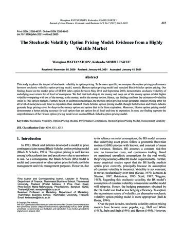
Woraphon WATTANATORN, Kedwadee SOMBULTAWEE /Journal of Asian Finance, Economics and Business Vol 8 No 2 (2021) 0685–0695688In the Thai market as well as other emerging market study, themarket liquidity issues is an important concern (Wattanatorn,Padungsaksawasdi, Chunhachinda, & Nathaphan, 2020;Wattanatorn & Tansupswatdikul, 2019). Therefore, we takecare of this liquidity issue following Bakshi et al. (1997). Wefurther class further classify our sample into six groups basedon day to expiration between seven days and two monthssince the near expiration options are more likely to sufferfrom liquidity-related bias to alleviate the liquidity-relatedbias concern. Table 2 shows the average option value andnumber of samples after the time-to-expiration criterion isused as a filter. Panel A shows the call options while PanelB shows the put options. There were a total of 2,220 optionprices, comprised of 1,060 call prices and 1,160 put prices.Both call and put options are more likely to trade at ATM.There are 425 call option traded at ITM and DITM whilethere are 323 option traded at OTM and DOTM. Also, wefind a similar trend for put option.3.2. Model Estimation and CalibrationTo estimate model parameters, we apply modelcalibration technique to accurately estimate Heston model’sparameters. The objective of model calibration is to obtainthe best fit model parameter which yield minimum differentbetween model predicted price and market prices (Bakshi etal., 1997; Beliaeva & Sanjay, 2010; Cui, del Baño Rollin, &Germano, 2017). As suggested by prior studies, we apply theminimize sum-square-error (SSE) between the market price,Cmkt, and model price, Cheston, as shown:error(σ, n, k, q, l, r) Cmkt – Cheston(St, T, K, Rf ; σ, n, k, q, l, r) (4)NSSE min error (σ, n, k, q, l, r) 2 (5)n 1For each day, we minimize the objective function showsin Eq. 5 and employ numerical method to estimate the valueof model parameter including σ, n, k, q, l, r. We then predictthe option price based on estimated parameter in next section.3.3. Model PerformanceTo compare the model performance between BlackSchole option pricing and Heston option pricing, weemploy two methods to evaluate model performance. First,we employ the traditional model evaluation method – theroot means square error (RMSE) as our second modelperformance measurement (Bakshi et al., 1997; Bhat, 2019;Singh & Dixit, 2016). RMSE is the absolute fit of the modeland market date. The notorious advantage of RMSE is thatthe RMSE squares the error term. Hence, RMSE gives thegreater weight to large error and thus penalized the largeerror model. As the result, RMSE reduces the tendencytoward overfit of the model. And we expect the better modelcan show low RMSE, which reflect the good fit of the model. (CnRMSE 1mkt Cmodel )n2(6)Second, we apply mean pricing error (MPE) to gauge themodel performance (Bakshi et al., 1997; Bhat, 2019; Feng,Hung, & Wang, 2016). MPE is the mean percentage pricedifferent between the mean actual market price and modelprice as shown in Eq. 6. Since MPE based their calculation onthe actual value, MPE can indicate the direction of biasnessfrom the model (Bhat, 2019; Wilson & Keating, 2001).MPE 1 n Cmkt Cmodel Cn 1mkt (7)4. Results and Discussion4.1. Summary statisticIn this section, we report the empirical finding of the study.Table 2 reports basic summary statistic of the sample understudy. Table 2 report cross-sectional option price and standarddeviation for each level of moneyness and time to expiration.Panel A shows the result for call option. The table shows thatthe value of option increase as it becomes in-the-money. Inaddition, the value of call option declines as it approachesthe expiration date. In a similar pattern, we find that the valueof put option increase as it becomes in-the-money option aswell as it increases as if the option is far from expiration date.4.2. Volatility SmileIn this section, we demonstrate the existence ofstochastic volatility. Figure 1 illustrates a clear picture ofstochastic volatility in SET50 index for call option. We findthat both BS implied volatility and Heston implied volatilityvary by the level of moneyness at all time to expiration.The existence of this smile volatility violates the basicassumption of BS model. Hence, our finding – the longestprior of study in Thailand, confirms the existing of smilevolatility in SET50 index in Thailand. We further comparethe smile volatility for BS and Heston model. We find thatthe BS demonstrates larger curvature than the Heston modelat all time to expiration. In addition, Figure 2 shows similarpattern of volatility smile for put option.
Woraphon WATTANATORN, Kedwadee SOMBULTAWEE /Journal of Asian Finance, Economics and Business Vol 8 No 2 (2021) 0685–0695689Table 2: Reports cross-sectional average of option price and number of samples (parenthesis). The sample period spansMay 2011 – September 2020. The samples are classified into five moneyness categories and six times to expiration. Panel Areport the sample average for call option and Panel B report the sample average for put optionPanel A: Call optionMoneynessDOTM(S/K 0.94)OTM(0.94 S/K 0.97)ATM(0.97 S/K 1.03)ITM(1.03 S/K 1.06)DITM(S/K 1.06)Day to 51)(42.528)Panel B: Put optionMoneynessDOTMOTM(K/S 0.94)(0.94 K/S 0.97)ATM(0.97 K/S 1.03)ITM(1.03 K/S 1.06)DITM(K/S 1.06)Day to (56.288)(32.002)Furthermore, we find that the volatility smile becomesmore severe as options approach their expiration for bothcall and put option. Figure 1 and Figure 2 show that thevolatility is flatter for 60 days before expiration than the nearexpiration. Clearly, it becomes more curvature, particularly at7 and 10 days before expiration. Also, the volatility is higherfor OTM option than ATM and ITM. In addition, we findthat BS volatility shows larger curvature than Heston modelin all time to expiration. As BS based their pricing modelon the assumption of constant volatility, we conjecture thatBS model faces a more severe in model mispricing. Hence,the Heston option pricing model – the alternative optionpricing which can accommodate the changing volatility canaccommodate this problem due to an ability of the model thatallows volatility to move stochastically over time. Therefore,the Heston model may improve pricing and hedgingperformance when trading options on the Thai market4.3. Parameter EstimationWe further estimate and calibrate Heston model’sparameters. We employ the method shown in section 3.2 toestimate the six-model parameter including s , v, k , q , l , rwhich are volatility of variance, level of volatility, meanreversion speed, mean reversion of variance, Volatilityrisk premium, and correlation coefficient between Weinerprocess respectively. We then report the result of estimationand calibration in Table 3 and Table 4.
690Woraphon WATTANATORN, Kedwadee SOMBULTAWEE /Journal of Asian Finance, Economics and Business Vol 8 No 2 (2021) 0685–0695Figure 1: Shows implied volatility to level of moneyness for call options at 7, 10, 15, 20, 40, and 60 day to expirationSource: AuthorFigure 2: Shows implied volatility to level of moneyness for put options at 7, 10, 15, 20, 40, and 60 day to expirationSource: Author
Woraphon WATTANATORN, Kedwadee SOMBULTAWEE /Journal of Asian Finance, Economics and Business Vol 8 No 2 (2021) 0685–0695691Table 3: Shows parameters for call options by time to expirationDays to 600.1604.0440.0000.19512.8740.606Table 4: Reports the model’s put option parameters for each time to expirationDays to .1052.4420.0000.82513.8620.219Table 3 shows the estimated parameter for call option.The results show that the speed of convergence, levelof long-run volatility, and volatility of variance falls asoption approach expiration date. Furthermore, the positivecorrelation for two Weiner processes suggests that therisk from the stochastic movement of the underlying assetand stochastic volatility move in the same direction, andthe impact of both risks moves closely as options approachexpiration.Table 4 reports the result for put option. We find that thelevel of variance increases as options approach expiration.The results are consistent with the results found in Figure 2.As options approach expiration, all else remaining equal,they become more volatile. The level of volatility (V0)increases as the options expire; the volatility of variance(sigma) representing the long-run mean of variance likewiseincreases. These findings support the hypothesis of highvolatility closer to expiration.4.4. Model PerformanceTable 5 compares option pricing performance betweenBS and Heston option pricing mode using MPE and RMSE.The finding in this section demonstrates that the Hestonmodel outperforms the BS model for all times to expirationand all degrees of moneyness. Panel A shows that both BSand Heston model provide a good result of pricing for OTMand DOTM option for all expiration periods. For example, at7 days prior expiration, Heston gives only 1.040% error onDOTM option pricing comparing with 2.028% generate by BSmodel. However, this superior performance decline for longerdays to expiration. For example, at 60 days prior expiration,Heston generates 4.013% prediction error comparing with4.297% predicted by BS model for the same DOTM option.Although we find that the Heston option pricing yields a betterpricing result in all level of moneyness and time to expiration,we further find that as option moves to ITM and DITM, thesuperior performance of Heston option pricing declines. Forexample, at 7 days prior expiration, Heston provides 37.298%pricing error for DITM option while BS generates 38.856%pricing error. Moreover, the superior performance declines forlonger day to expiration as we found in DOTM. Moreover,the results show that both BS and Heston model generatelarge pricing error for the longer day to expiration option. Onepossible explanation of this large error is the liquidity issuesupported by several studies (Brenner, Eldor, & Hauser, 2001;Peña et al., 1999). In addition, this liquidity issue is found tobe an important issue in the Thai market (Pojanavatee, 2020;Wattanatorn et al., 2020).Consistent with Panel A, the findings for put optionshown in Panel B provide the similar results. Although,Heston model for put option provides lower pricing error inall level of moneyness and time to expiration like call option,we find that the levels of error are not far better than BSlike in call option pricing. This findings are similar to thoseof call option. In sum, our results demonstrate the superior
Woraphon WATTANATORN, Kedwadee SOMBULTAWEE /Journal of Asian Finance, Economics and Business Vol 8 No 2 (2021) 0685–0695692performance of the Heston model over BS in emergingmarket context. The findings here are consistent with theevidence found in develop markets (Bakshi et al., 1997;Fiorentini et al., 2002). Also, we find the same superiorperformance of Heston model over BS as in Indian stockindex option (Singh & Dixit, 2016). More recently, ourresults go along with Bhat (2019) who shows the superiorpricing performance of Heston model over BS model incurrency option.Table 6 reports the result of model performance basedon MPE. Panel A reports the result for call option whilePanel B reports the result for put option. Consistencewith prior section, in Panel A, we find that Heston modeloutperforms BS model for all level of moneyness and timeto expiration. Based on MPE, we can see the direction ofbias of pricing error. The result reported by Table 6 clearlyshows that the Heston option pricing model predictspricing error toward undervaluing. Unlike Heston model,the BS model provides overvalue estimation for allmoneyness and time to expiration. Although in previoussection we find the RMSE are large for both the Hestonand BS model, MPE is obviously lower for Heston model.In Panel B, we find the similar results for put option.Table 5: Reports model pricing performance-based root mean square error—RMSE (Eq. 6). Panel A reports the result for calloption while Panel B report the result for put optionPanel A: Call optionMoneynessDOTMOTMATMModelDay to Panel B: Put optionMoneynessModelDay to 27946.321BS40.69033.36160.27073.08275.51857.556
Woraphon WATTANATORN, Kedwadee SOMBULTAWEE /Journal of Asian Finance, Economics and Business Vol 8 No 2 (2021) 0685–0695693Table 6: Reports model pricing performance based on mean pricing error—MPE (Eq. 7). Panel A reports the result for calloption while Panel B report the result for put optionPanel A: Call optionMoneynessDOTMOTMATMDay to .02531.74849.44867.791Panel B: Put optionMoneynessDOTMOTMDay to 0.00710.3743.0647.8005. ConclusionIn general, derivatives are widely used as an instrumentto manage risk (Park & Park, 2020) while the one of themost popular instrument used to manage portfolio risk isan option on
pricing model can replicate the market price, volatility-based option pricing models such as the Heston model and Deterministic Volatility Function (DVF) are among the best estimation models compared with other option pricing further examine the effect of volatility smiles on the SET50 index using both put and call options. 2.2. Stochastic .