WIXLIB

A 3-month call optionConsider a 3-month call option on the stock with a strike of 21.Backward induction: Given the terminal stock price (ST ), we can computethe option payoff at each node, (ST K ) .The zero-coupon bond price with 1 par valueBT ST Bt 0.9704 cT QSt 20QQct ?Q BT ST cT is: 1 e .12 .25 0.9704.12211180Two angles:Replicating: See if you can replicate the call’s payoff using stock and bond. If the payoffs equal, so does the value.Hedging: See if you can hedge away the risk of the call using stock. Ifthe hedged payoff is riskfree, we can compute the present value usingriskfree rate. . . . . . . . . . . . . . . .Liuren Wu (Baruch)Option Pricing Introduction. . . . . . . . . . . . .Options Markets. . . . .15 / 78

ReplicatingBT 1 ST 22Bt 0.9704 cT 1QSt 20QQct ?Q BT 1ST 18cT 0Assume that we can replicate the payoff of 1 call using share of stock andD par value of bond, we have1 22 D1,0 18 D1.Solve for : (1 0)/(22 18) 1/4. Change in C/Change in S,a sensitivity measure.Solve for D: D 14 18 4.5 (borrow).Value of option value of replicating portfolio 14 20 4.5 0.9704 0.633. .Liuren Wu (Baruch)Option Pricing Introduction. . . . . . . . . . . . . . . . . . . . . . . . . . .Options Markets. . . . .16 / 78

HedgingBT 1 ST 22Bt 0.9704 cT 1QSt 20QQct ?Q BT 1ST 18cT 0Assume that we can hedge away the risk in 1 call by shorting share ofstock, such as the hedged portfolio has the same payoff at both nodes:1 22 0 18.Solve for : (1 0)/(22 18) 1/4 (the same): Change in C/Change in S, a sensitivity measure.The hedged portfolio has riskfree payoff: 1 41 22 0 14 18 4.5.Its present value is: 4.5 0.9704 4.3668 1ct St .ct 4.3668 St 4.3668 14 20 0.633. .Liuren Wu (Baruch)Option Pricing Introduction. . . . . . . . . . . . . . . . . . . . . . . . . . .Options Markets. . . . .17 / 78

One principle underlying two anglesIf you can replicate, you can hedge:Long the option contract, short the replicating portfolio.The replication portfolio is composed of stock and bond.Since bond only generates parallel shifts in payoff and does not play any rolein offsetting/hedging risks, it is the stock that really plays the hedging role.The optimal hedge ratio when hedging options using stocks is defined as theratio of option payoff change over the stock payoff change — Delta.Hedging derivative risks using the underlying security (stock, currency) iscalled delta hedging.To hedge a long position in an option, you need to short delta of theunderlying.To replicate the payoff of a long position in option, you need to longdelta of the underlying. .Liuren Wu (Baruch)Option Pricing Introduction. . . . . . . . . . . . . . . . . . . . . . . . . . .Options Markets. . . . .18 / 78

The limit of delta hedgingDelta hedging completely erases risk under the binomial model assumption:The underlying stock can only take on two possible values.Using two (different) securities can span the two possible realizations.We can use stock and bond to replicate the payoff of an option.We can also use stock and option to replicate the payoff of a bond.One of the 3 securities is redundant and can hence be priced by theother two.What will happen for the hedging/replicating exercise if the stock can takeon 3 possible values three months later, e.g., (22, 20, 18)?It is impossible to find a that perfectly hedge the option position orreplicate the option payoff.We need another instrument (say another option) to do perfecthedging or replication. .Liuren Wu (Baruch)Option Pricing Introduction. . . . . . . . . . . . . . . . . . . . . . . . . . .Options Markets. . . . .19 / 78

Introduction to risk-neutral valuationp BT 1 ST 22Bt 0.9704 QQSt 20QQ BT 11 pST 18Compute a set of artificial probabilities for the two nodes (p, 1 p) suchthat the stock price equals the expected value of the terminal payment,discounted by the riskfree rate.20 0.9704 (22p 18(1 p)) p 20/0.9704 1822 18 0.6523Since we are discounting risky payoffs using riskfree rate, it is as if we live inan artificial world where people are risk-neutral. Hence, (p, 1 p) are therisk-neutral probabilities.These are not really probabilities, but more like unit prices:0.9704p is theprice of a security that pays 1 at the up state and zero otherwise.0.9704(1 p) is the unit price for the down state.To exclude arbitrage, the same set of unit prices (risk-neutral probabilities). . . . . . . . . . . . . . . .should be applicable to all securities, including options. . . . . . . . . . . . . . . . . .Liuren Wu (Baruch)Option Pricing IntroductionOptions Markets. .20 / 78

Risk-neutral probabilitiesUnder the binomial model assumption, we can identify a unique set ofrisk-neutral probabilities (RNP) from the current stock price.The risk-neutral probabilities have to be probability-like (positive, lessthan 1) for the stock price to be arbitrage free.What would happen if p 0 or p 1?If the prices of market securities do not allow arbitrage, we can identify atleast one set of risk-neutral probabilities that match with all these prices.When the market is, in addition, complete (all risks can be hedged awaycompletely by the assets), there exist one unique set of RNP.Under the binomial model, the market is complete with the stock alone. Wecan uniquely determine one set of RNP using the stock price alone.Under a trinomial assumption, the market is not complete with the stockalone: There are many feasible RNPs that match the stock price.In this case, we add an option to fully determine a unique set of RNP.That is, we use this option (and the trinomial) to complete the market. .Liuren Wu (Baruch)Option Pricing Introduction. . . . . . . . . . . . . . . . . . . . . . . . . . .Options Markets. . . . .21 / 78

Market completenessMarket completeness (or incompleteness) is a relative concept: Market maynot be complete with one asset, but can be complete with two.To me, the real-world market is severely incomplete with primary marketsecurities alone (stocks and bonds).To complete the market, we need to include all available options, plus modelstructures.Model and instruments can play similar rules to complete a market.RNP are not learned from the stock price alone, but from the option prices.Risk-neutral dynamics need to be estimated using option prices.Options are not redundant.Caveats: Be aware of the reverse flow of information and supply/demandshocks. .Liuren Wu (Baruch)Option Pricing Introduction. . . . . . . . . . . . . . . . . . . . . . . . . . .Options Markets. . . . .22 / 78

Muti-step binomial treesA one-step binomial model looks very Mickey Mouse: In reality, the stockprice can take on many possible values than just two.Extend the one-step to multiple steps. The number of possible values(nodes) at expiry increases with the number of steps.With many nodes, using stock alone can no longer achieve a perfect hedgein one shot.But locally, within each step, we still have only two possible nodes. Thus,we can achieve perfect hedge within each step.We just need to adjust the hedge at each step — dynamic hedging.By doing as many hedge rebalancing at there are time steps, we can stillachieve a perfect hedge globally.The market can still be completed with the stock alone, in a dynamic sense.A multi-step binomial tree can still still very useful in practice in, forexample, handling American options, discrete dividends, interest rate termstructures . . . . . . . . . . . . . . . .Liuren Wu (Baruch)Option Pricing Introduction. . . . . . . . . . . . .Options Markets. . . . .23 / 78

Constructing the binomial tree St u fuSt Qft QSdQQ tfdOne way to set up the tree is to use (u, d) to match the stock returnvolatility (Cox, Ross, Rubinstein):u eσ t,d 1/u.σ— the annualized return volatility (standard deviation).The risk-neutral probability becomes: p a du dwherer ta efor non-dividend paying stock.a e (r q) t for dividend paying stock.a e (r rf ) t for currency.a 1 for futures.Liuren Wu (Baruch)Option Pricing Introduction. . . . . . . . . . . . . . . . . . . . . . . . . . . .Options Markets. . . . .24 / 78

Estimating the return volatility σTo determine the tree (St , u, d), we setu eσ t,d 1/u.The only un-observable or “free” parameter is the return volatility σ.Mean expected return (risk premium) does not matter for derivativepricing under the binomial model because we can completely hedgeaway the risk.St can be observed from the stock market.We canthe return volatility using the time series data: estimate[] N111σb t N 1 t 1 (Rt R)2 . tis for annualization.Implied volatility: We can estimate the volatility (σ) by matching observedoption prices. .Liuren Wu (Baruch)Option Pricing Introduction. . . . . . . . . . . . . . . . . . . . . . . . . . .Options Markets. . . . .25 / 78

The Black-Merton-Scholes (BMS) modelBlack and Scholes (1973) and Merton (1973) derive option prices under thefollowing assumption on the stock price dynamics,dSt µSt dt σSt dWtThe binomial model: Discrete states and discrete time (The number ofpossible stock prices and time steps are both finite).The BMS model: Continuous states (stock price can be anything between 0and ) and continuous time (time goes continuously).BMS proposed the model for stock option pricing. Later, the model hasbeen extended/twisted to price currency options (Garman&Kohlhagen) andoptions on futures (Black).I treat all these variations as the same concept and call themindiscriminately the BMS model. .Liuren Wu (Baruch)Option Pricing Introduction. . . . . . . . . . . . . . . . . . . . . . . . . . .Options Markets. . . . .26 / 78

Primer on continuous time processdSt µSt dt σSt dWtThe driver of the process is Wt , a Brownian motion, or a Wiener process.The sample paths of a Brownian motion are continuous over time, butnowhere differentiable.It is the idealization of the trajectory of a single particle beingconstantly bombarded by an infinite number of infinitessimally smallrandom forces.Like a shark, a Brownian motion must always be moving, or else it dies.If you sum the absolute values of price changes over a day (or any timehorizon) implied by the model, you get an infinite number.If you tried to accurately draw a Brownian motion sample path, yourpen would run out of ink before one second had elapsed. .Liuren Wu (Baruch)Option Pricing Introduction. . . . . . . . . . . . . . . . . . . . . . . . . . .Options Markets. . . . .27 / 78

Properties of a Brownian motiondSt µSt dt σSt dWtThe process Wt generates a random variable that is normallydistributed with mean 0 and variance t, ϕ(0, t). (Also referred to as Gaussian.)Everybody believes in the normal approximation, theexperimenters because they believe it is a mathematical theorem,the mathematicians because they believe it is an experimentalfact!The process is made of independent normal increments dWt ϕ(0, dt).“d” is the continuous time limit of the discrete time difference ( ). t denotes a finite time step (say, 3 months), dt denotes an extremelythin slice of time (smaller than 1 milisecond).It is so thin that it is often referred to as instantaneous.Similarly, dWt Wt dt Wt denotes the instantaneous increment(change) of a Brownian motion.By extension, increments over non-overlapping time periods areindependent: For (t1 t2 t3 ), (Wt3 Wt2 ) ϕ(0, t3 t2 ) is independent. . . . . . . . . . . . . . . . .of (Wt2 Wt1 ) ϕ(0, t2 t1 ). . . . . . . . . . . . . . . . . . .Liuren Wu (Baruch)Option Pricing IntroductionOptions Markets28 / 78.

Properties of a normally distributed random variabledSt µSt dt σSt dWtIf X ϕ(0, 1), then a bX ϕ(a, b 2 ).If y ϕ(m, V ), then a by ϕ(a bm, b 2 V ).Since dWt ϕ(0, dt), the instantaneous price changedSt µSt dt σSt dWt ϕ(µSt dt, σ 2 St2 dt).The instantaneous returndSS µdt σdWt ϕ(µdt, σ 2 dt).Under the BMS model, µ is the annualized mean of the instantaneousreturn — instantaneous mean return.σ 2 is the annualized variance of the instantaneous return —instantaneous return variance.σ is the annualized standard deviation of the instantaneous return —instantaneous return volatility. .Liuren Wu (Baruch)Option Pricing Introduction. . . . . . . . . . . . . . . . . . . . . . . . . . .Options Markets. . . . .29 / 78

Geometric Brownian motiondSt /St µdt σdWtThe stock price is said to follow a geometric Brownian motion.µ is often referred to as the drift, and σ the diffusion of the process.Instantaneously, the stock price change is normally distributed,ϕ(µSt dt, σ 2 St2 dt).Over longer horizons, the price change is lognormally distributed.The log return (continuous compounded return) is normally distributed overall horizons:)(d ln St µ 12 σ 2 dt σdWt . (By Ito’s lemma)d ln St ϕ(µdt 12 σ 2 dt, σ 2 dt).ln St ϕ(ln S0(( µt 12)σ 2 t, σ 2 t).)ln ST /St ϕ µ 12 σ 2 (T t), σ 2 (T t) .1Integral form: St S0 e µt 2 σ2t σWt,ln St ln S0 µt 12 σ 2 t σWt. .Liuren Wu (Baruch)Option Pricing Introduction. . . . . . . . . . . . . . . . . . . . . . . . . . .Options Markets. . . . .30 / 78

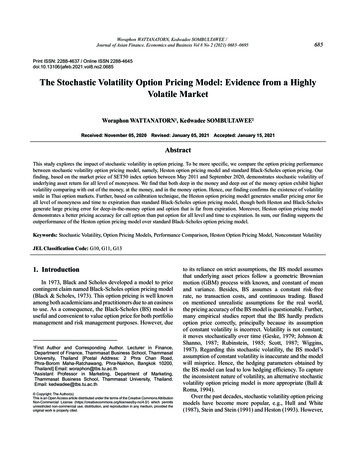
Normal versus lognormal distributionµ 10%, σ 20%, S0 100, t 1.20.021.80.0181.60.0161.40.0141.20.012PDF of StPDF of ln(St/S0)dSt µSt dt σSt dWt ,10.80.010.0080.60.0060.40.0040.20.0020 1 0.50ln(St/S0)0.51S0 100050100150St200250The earliest application of Brownian motion to finance is by Louis Bachelier in hisdissertation (1900) “Theory of Speculation.” He specified the stock price asfollowing a Brownian motion with drift:dSt µdt σdWt. .Liuren Wu (Baruch)Option Pricing Introduction. . . . . . . . . . . . . . . . . . . . . . . . . . .Options Markets. . . . .31 / 78

Simulate 100 stock price sample pathsdSt µSt dt σSt dWt ,µ 10%, σ 20%, S0 100, t 1.2000.050.041800.03160Stock priceDaily returns0.020.010140120 0.01100 0.0280 0.03 Stock with the return process: d ln St (µ 12 σ 2 )dt σdWt .Discretize to daily intervals dt t 1/252.Draw standard normal random variables ε(100 252) ϕ(0, 1). Convert them into daily log returns: Rd (µ 12 σ 2 ) t σ tε.Convert returns into stock price sample paths: St S0 e. .Liuren Wu (Baruch)Option Pricing Introduction 252d 1Rd. . . . . . . . . . . . . . . . . . . . . . . . . . .Options Markets. . . . .32 / 78

Ito’s lemma on continuous processesGiven a dynamics specification for xt , Ito’s lemma determines the dynamics ofany functions of x and time, yt f (xt , t). Example: Given dynamics on St ,derive dynamics on ln St /S0 .For a generic continuous process xt ,dxt µx dt σx dWt ,the transformed variable y f (x, t) follows,()12dyt ft fx µx fxx σx dt fx σx dWt2You can think of it as aTaylor expansion up to dt term, with (dW )2 dtExample 1:( dSt µS) t dt σSt dWt and y ln St . We haved ln St µ 12 σ 2 dt σdWt Example 2: dvt κ (θ vt ) dt ω vt dWt , and σt vt .()1 1111dσt σt κθ κσt ω 2 σt 1 dt ωdWt2282Example 3: dxt κxt dt σdWt and vt a .bx. t2. . . dvt ?. . . . . . . . . .Liuren Wu (Baruch)Option Pricing Introduction. . . . . . . . . . . . . .Options Markets. . . . .33 / 78

Ito’s lemma on jumpsFor a generic process xt with jumps,dxt µx dt σx dWt g (z) (µ(dz, dt) ν(z, t)dzdt) , (µx Et [g ]) dt σx dWt g (z)µ(dz, dt),where the random counting measure µ(dz, dt) realizes to a nonzero value for agiven z if and only if x jumps from xt to xt xt g (z) at time t. The processν(z, t)dzdt compensates the jump process so that the last term is the incrementof a pure jump martingale. The transformed variable y f (x, t) follows,()dyt ft fx µx 21 fxx σx2 dt fx σx dWt ( (f (xt g (z), t) 1f (xt 2 ,)t)) µ(dz, dt) fx g (z)ν(z, t)dzdt, ft fx (µx Et [g ]) 2 fxx σx dt fx σx dWt (f (xt g (z), t) f (xt , t)) µ(dz, dt). .Liuren Wu (Baruch)Option Pricing Introduction. . . . . . . . . . . . . . . . . . . . . . . . . . .Options Markets. . . . .34 / 78

Ito’s lemma on jumps: Merton (1976) exampledyt ()ft fx µx 12 fxx σx2 dt fx σx dWt µ(dz, dt) fx g (z)ν(z, t)dzdt,( (f (xt g (z), t) f (x1t , t)))ft fx (µx Et [g (z)]) 2 fxx σx2 dt fx σx dWt (f (xt g (z), t) f (xt , t)) µ(dz, dt)Merton (1976)’s jump-diffusion process: dSt µSt dt σSt dWt St (e z 1) (µ(z, t) ν(z, t)dzdt) , andy ln St . We have() 1d ln St µ σ 2 dt σdWt zµ(dz, dt) (e z 1) ν(z, t)dzdt2f (xt g (z), t) f (xt , t) ln St ln St ln(St e z ) ln St z.The specification (e z 1) on price guarantees that the maximum downsidejump is no larger than the pre-jump price level St .In Merton, ν(z, t) λ σLiuren Wu (Baruch)1 J2πe (z µJ )22σ 2J.Option Pricing Introduction. . . . . . . . . . . . . . . . . . . . . . . . . . . .Options Markets. . . . .35 / 78

The key idea behind BMS option pricingUnder the binomial mode

6. implied volatility surface Liuren Wu (Baruch) Option Pricing Introduction Options Markets 2 / 78. Review: Valuation and investment in primary securities . Liuren Wu (Baruch) Option Pricing Introduction Options Markets 14 / 78. A 3-month call option Consider a 3-month call option on the stock with a strike of 21. .