WIXLIB

Freescale Semiconductor, Inc.Application NoteDocument Number: AN4255Rev. 4, 07/2015FFT-Based Algorithm for MeteringApplicationsby: Ludek Slosarcik1IntroductionThe Fast Fourier Transform (FFT) is a mathematicaltechnique for transforming a time-domain digital signal intoa frequency-domain representation of the relative amplitudeof different frequency regions in the signal. The FFT is amethod for doing this process very efficiently. It may becomputed using a relatively short excerpt from a signal.The FFT is one of the most important topics in Digital SignalProcessing. It is extremely important in the area of frequency(spectrum) analysis; for example, voice recognition, digitalcoding of acoustic signals for data stream reduction in thecase of digital transmission, detection of machine vibration,signal filtration, solving partial differential equations, and soon.This application note describes how to use the FFT inmetering applications, especially for energy computing inpower meters. The critical task in a metering application isan accurate computation of energies, which are sometimesreferred to as billing quantities. Their computation must becompliant with the international standard for electronicmeters. The remaining quantities are calculated forinformative purposes and they are referred to as non-billing. 2015 Freescale Semiconductor, Inc. All rights reserved.1.2.3.4.5.6.7.8.ContentsIntroduction . . . . . . . . . . . . . . . . . . . . . . . . . . . . . . . . . 1DFT basics . . . . . . . . . . . . . . . . . . . . . . . . . . . . . . . . . 2FFT implementation . . . . . . . . . . . . . . . . . . . . . . . . . . 3Using FFT for power computing . . . . . . . . . . . . . . . . 9Metering library . . . . . . . . . . . . . . . . . . . . . . . . . . . . 13Summary . . . . . . . . . . . . . . . . . . . . . . . . . . . . . . . . . . 41References . . . . . . . . . . . . . . . . . . . . . . . . . . . . . . . . . 42Revision history . . . . . . . . . . . . . . . . . . . . . . . . . . . . 42

DFT basics2DFT basicsFor a proper understanding of the next sections, it is important to clarify what a Discrete Fourier Transform(DFT) is. The DFT is a specific kind of discrete transform, used in Fourier analysis. It transforms onefunction into another, which is called the frequency-domain representation of the original function(a function in the time domain). The input to the DFT is a finite sequence of real or complex numbers,making the DFT ideal for processing information stored in computers. The relationship between the DFTand the FFT is as follows: DFT refers to a mathematical transformation or function, regardless of how itis computed, whereas the FFT refers to a specific family of algorithms for computing a DFT.The DFT of a finite-length sequence of size N is defined as follows:N–1X k x n en 02 nk– j ------------NN–1 2 nk2 nkx n cos ------------- – j x n sin ------------- N N Eqn. 1n 00 k NWhere: X(k) is the output of the transformation x(n) is the input of the transformation (the sampled input signal) j is the imaginary unitEach item in Equation 1 defines a partial sinusoidal element in complex format with a kF0 frequency,with (2 nk/N) phase, and with x(n) amplitude. Their vector summation for n 0,1,.,N-1 (see Equation 1)and for the selected k-item, represents the total sinusoidal item of spectrum X(k) in complex format forthe kF0 frequency. Note, that F0 is the frequency of the input periodic signal. In the case of non-periodicsignals, F0 means the selected basic period of this signal for DFT computing.The Inverse Discrete Fourier Transform (IDFT) is given by:N–11x n ---- N X k e2 nkj ------------NEqn. 2k 00 n NThanks to Equation 2, it is possible to compute discrete values of x(n) from the spectrum items of X(k)retrospectively.In these two equations, both X(k) and x(n) can be complex, so N complex multiplications and (N-1)complex additions are required to compute each value of the DFT if we use Equation 1 directly.Computing all N values of the frequency components requires a total of N2 complex multiplications andN (N-1) complex additions.FFT-Based Algorithm for Metering Applications, Application Note, Rev. 4, 07/20152Freescale Semiconductor, Inc.

FFT implementation3FFT implementationWith regards to the derived equations in Section 2, “DFT basics,” it is good to introduce the followingsubstitution:WNnk e2 nk– j ------------NEqn. 3The WNnk element in this substitution is also called the “twiddle factor.” With respect to this substitution,we may rewrite the equation for computing the DFT and IDFT into these formats:N–1DFT x n X k x n WnkEqn. 4Nn 0N–1 X k W1IDFT X k x n ---- N–n kNEqn. 5k 0To improve efficiency in computing the DFT, some properties of WNnk are exploited. They are describedas follows:Symmetral property:WNnk N 2 –WNnkEqn. 6Periodicity property:WNnk WNnk N WNnk 2N Eqn. 7Recursion property:WN 2nk WN2nkEqn. 8These properties arise from the graphical representation of the twiddle factor (Equation 4) by the rotationalvector for each nk value.3.1The radix-2 decimation in time FFT descriptionThe basic idea of the FFT is to decompose the DFT of a time-domain sequence of length N intosuccessively smaller DFTs whose calculations require less arithmetic operations. This is known asa divide-and-conquer strategy, made possible using the properties described in the previous section.The decomposition into shorter DFTs may be performed by splitting an N-point input data sequence x(n)into two N/2-point data sequences a(m) and b(m), corresponding to the even-numbered and odd-numberedsamples of x(n), respectively, that is: a(m) x(2m), that is, samples of x(n) for n 2m b(m) x(2m 1), that is, samples of x(n) for n 2m 1where m is an integer in the range of 0 m N/2.FFT-Based Algorithm for Metering Applications, Application Note, Rev. 4, 07/2015Freescale Semiconductor, Inc.3

FFT implementationThis process of splitting the time-domain sequence into even and odd samples is what gives the algorithmits name, “Decimation In Time (DIT)”. Thus, a(m) and b(m) are obtained by decimating x(n) by a factorof two; hence, the resulting FFT algorithm is also called “radix-2”. It is the simplest and most commonform of the Cooley-Tukey algorithm [1].Now, the N-point DFT (see Equation 1) can be expressed in terms of DFTs of the decimated sequencesas follows:N 2–1N–1X k x n Wnk Nn 0 N 2–1x 2m W N2mk m 0 2m 1 k Eqn. 9m 0N 2–1 x 2m 1 W NN 2–1x 2m W N2mk WNm 0k x 2m 1 W N2mkm 0With the substitution given by Equation 8, the Equation 9 can be expressed as:N 2–1X k N 2–1a m WN 2mk WNm 0k b m WN 2mkk A k WN B k Eqn. 10m 00 k NThese two summations represent the N/2-point DFTs of the sequences a(m) and b(m), respectively.Thus, DFT[a(m)] A(k) for even-numbered samples, and DFT[b(m)] B(k) for odd-numbered samples.Thanks to the periodicity property of the DFT (Equation 7), the outputs for N/2 k N from a DFT oflength N/2 are identical to the outputs for 0 k N/2. That is, A(k N/2) A(k) and B(k N/2) B(k) for0 k N/2. In addition, the factor WNk N/2 WNk thanks the to symmetral property (Equation 6).Thus, the whole DFT can be calculated as follows:kX k A k WN B k kX k N 2 A k – WN B k Eqn. 110 k N 2This result, expressing the DFT of length N recursively in terms of two DFTs of size N/2, is the core ofthe radix-2 DIT FFT. Note, that final outputs of X(k) are obtained by a / combination of A(k) andB(k)WNk, which is simply a size 2 DFT. These combinations can be demonstrated by a simply-orientedgraph, sometimes called “butterfly” in this context (see Figure 1).X(k) A(k) WNkB(k)A(k)B(k)WNk-1X(k N/2) A(k)-WNkB(k)Figure 1. Basic butterfly computation in the DIT FFT algorithmFFT-Based Algorithm for Metering Applications, Application Note, Rev. 4, 07/20154Freescale Semiconductor, Inc.

FFT implementationThe procedure of computing the discrete series of an N-point DFT into two N/2-point DFTs may beadopted for computing the series of N/2-point DFTs from items of N/4-point DFTs. For this purpose, eachN/2-point sequence should be divided into two sub-sequences of even and odd items, and computing theirDFTs consecutively. The decimation of the data sequence can be repeated again and again until theresulting sequence is reduced to one basic 3)X(4)X(5)X(6)X(7)DFTstage 1stage 2stage 3Figure 2. Decomposition of an 8-point DFTFor illustrative purposes, Figure 2 depicts the computation of an N 8-point DFT. We observe thatthe computation is performed in three stages (3 log28), beginning with the computations of four 2-pointDFTs, then two 4-point DFTs, and finally, one 8-point DFT. Generally, for an N-point FFT, the FFTalgorithm decomposes the DFT into log2N stages, each of which consists of N/2 butterflycomputations.The combination of the smaller DFTs to form the larger DFT for N 8 is illustratedin Figure 3.FFT-Based Algorithm for Metering Applications, Application Note, Rev. 4, 07/2015Freescale Semiconductor, Inc.5

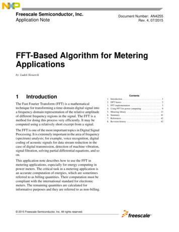
FFT implementationx(n)stage 1k 0stage 2k 0,1stage 3k 0,1,2,3W84k W2kW82k W4kW 8kX(k)X(0)x(0)x(4)W80X(1)-1W 80x(2)x(6)W 82W 80-1X(3)-1W80x(1)x(5)X(4)-1W 81W 80-1X(5)-1W82W 80x(3)x(7)X(2)-1-1W82W 80X(6)-1W83X(7)-1-1-1Figure 3. 8-point radix-2 DIT FFT algorithm data flowEach dot represents a complex addition and each arrow represents a complex multiplication, as shown inFigure 3. The WNk factors in Figure 3 may be presented as a power of two (W2) at the first stage, as a powerof four (W4) at the second stage, as a power of eight (W8) at the third stage, and so on. It is also possibleto represent it uniformly as a power of N (WN ), where N is the size of the input sequence x(n). The contextbetween both expressions is shown in Equation 8.3.2The radix-2 decimation in time FFT requirementsFor effective and optimal decomposition of the input data sequence into even and odd sub-sequences, it isgood to have the power-of-two input data samples (., 64, 128, and so on).The first step before computing the radix-2 FFT is re-ordering of the input data sequence (see also the leftside of Figure 2 and Figure 3). This means that this algorithm needs a bit-reversed data ordering; that is,the MSBs become LSBs, and vice versa. Table 1 shows an example of a bit-reversal with an 8-point inputsequence.Table 1. Bit reversal with an 8-point input sequenceDecimal number01234567Binary equivalent000001010011100101110111Bit reversed binary000100010110001101011111Decimal equivalent04261537FFT-Based Algorithm for Metering Applications, Application Note, Rev. 4, 07/20156Freescale Semiconductor, Inc.